Analysis in R: Easy to create color palettes and manipulate continuous and discrete scales “scales” package

This article introduces the scales package, which makes it easy to create color palettes, manage string display formats, and manage continuous and discrete scales. Using the continuous and discrete scale management commands, you can easily customize the axes and scales of the ggplot2 package.

This package is recommended for those unfamiliar with the operation of R.

Package version is 1.1.1. Checked with R version 4.2.2.

Install Package

Run the following command.

#Install Package
install.packages("scales")

Loading the library

Run the following command.

#Loading the library
library("scales")

Color palette creation commands

See the command and package help for details.

#Color palette creation:show_col command
#show_col(色, labels = show color code:TRUE/FALSE, borders = Specify border color: NA for no border)
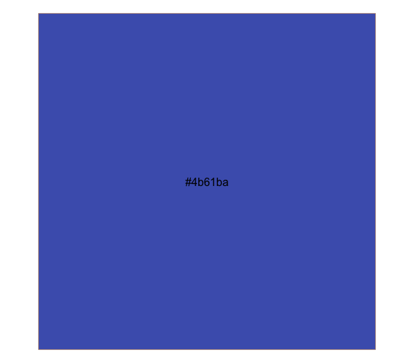
show_col("#4b61ba", labels = TRUE, borders = "#a87963")

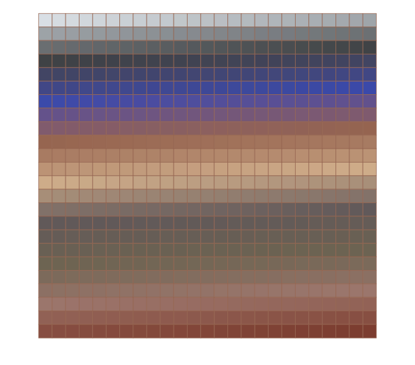
#Combination with seq_gradient_pal command
#Exsample:https://www.karada-good.net/analyticsr/r-83/
#Danmachi,Hanasaku Iroha Palette
x <- seq(0, 1, length = 600)
show_col(seq_gradient_pal(c("#e1e6ea", "#505457", "#4b61ba", "#a87963",
                            "#d9bb9c", "#756c6d", "#807765", "#ad8a80"))(x),
         labels = FALSE, borders = "#a87963")

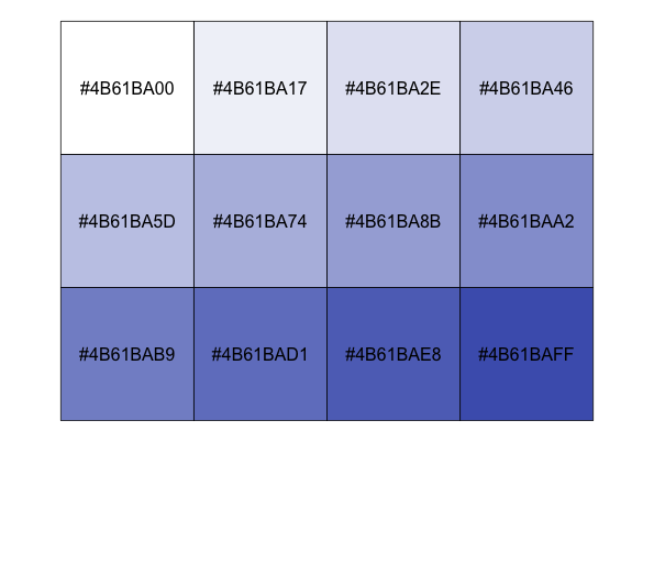
#Create a single color palette with a specified transparency:alpha command
#alpha(color, alpha = 0-1 as a single number or as an array)
show_col(alpha("#4b61ba", seq(0, 1, length = 12)))

Output Example

・show_col command

・Combination with seq_gradient_pal command

・alpha command

String display format and continuous and discrete scale commands

See the command and package help for details.

###Creating Data#####
TestData <- data.frame(Group = paste0("TEST", 1:10),
                       Data1 = sample(1:500, 10),
                       Data2 = sample(200:300, 10))
#####

#comma_format command
#Comma every 3 digits
comma(c(1, 1000, 2000, 1000000))
[1] "1" "1,000" "2,000" "1,000,000"

#Create breaks and labels for a specified range: cbreaks command
#"pretty_breaks" option: specifies the number of breaks
#"labels" option:default;scientific_format()
#Commands that can be set to label options
#comma display;comma_format(digits = 3), date display;date_format(format = "%Y-%m-%d", tz = "UTC"),
#dollar display;dollar_format(), expression expression;percent_format(), unit display;unit_format()
cbreaks(c(0, 100), pretty_breaks(10), labels = percent_format())
$breaks
[1]   0  10  20  30  40  50  60  70  80  90 100
$labels
[1] "0%" "1,000%" "2,000%" "3,000%" "4,000%" "5,000%" "6,000%" "7,000%" "8,000%" "9,000%" "10,000%"

#Breaks can also be set manually
cbreaks(c(0, 100), breaks = c(15, 30), labels = percent_format())
$breaks
[1] 15 30
$labels
[1] "1,500%" "3,000%"

#Continuous scale: cscale command
#Two palettes that could be used, see HELP for other palettes
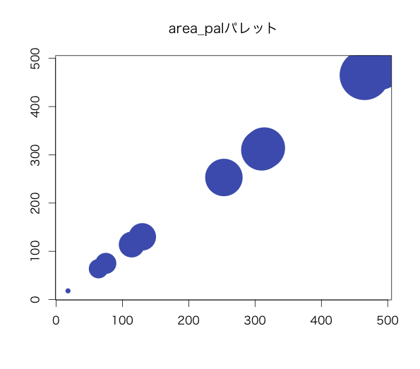
#area_pal palette
plot(TestData[, 2], TestData[, 2], xlab = "", ylab = "", main = "area_pal palette",
     cex = cscale(TestData[, 2], area_pal(range = c(1, 10))), col = "#4b61ba", pch = 16)
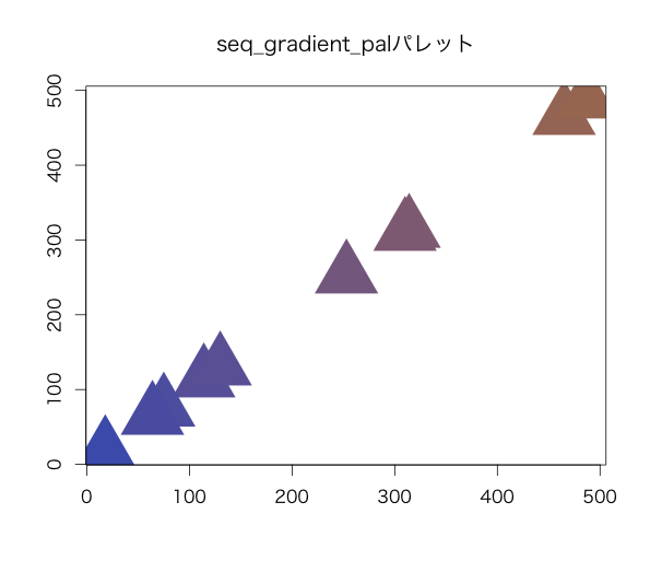
#seq_gradient_pal palette
plot(TestData[, 2], TestData[, 2], pch = 17, cex = 6, xlab = "", ylab = "", main = "seq_gradient_pal palette",
     col = cscale(TestData[, 2], seq_gradient_pal("#4b61ba", "#a87963")))

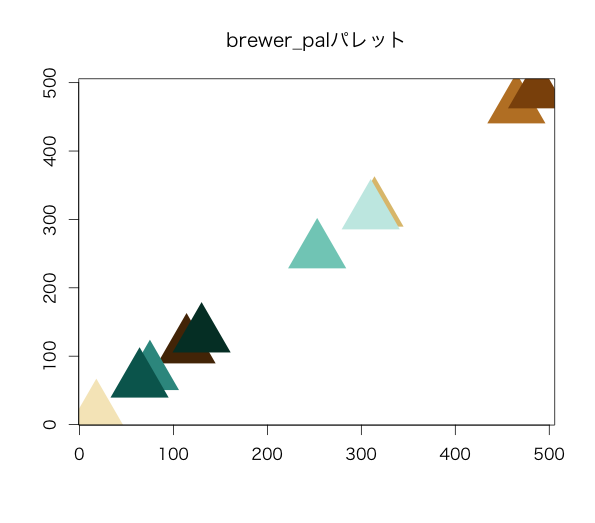
#Discrete scale: dscale command
#4 palettes that could be used, see HELP for other palettes
#brewer_pal palette
plot(TestData[, 2], TestData[, 2], pch = 17, cex = 6, xlab = "", ylab = "",
     main = "brewer_pal palette", col = dscale(TestData[, 1], brewer_pal("div")))
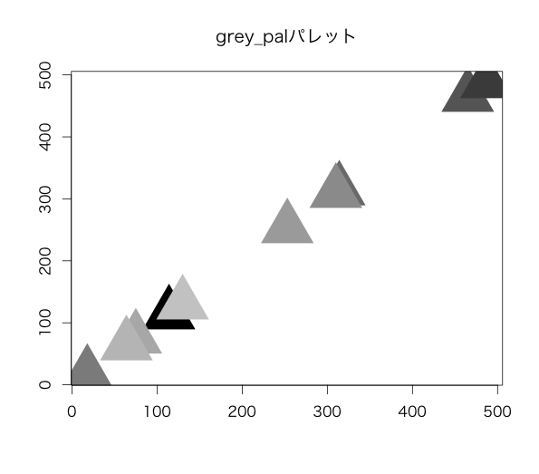
#grey_pal palette
plot(TestData[, 2], TestData[, 2], pch = 17, cex = 6, xlab = "", ylab = "", main = "grey_pal palette",
     col = dscale(TestData[, 1], grey_pal(start = 0, end = 0.8)))
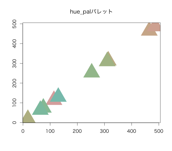
#hue_pal palette
#direction option:1 = clockwise, -1 = counter-clockwise
plot(TestData[, 2], TestData[, 2], pch = 17, cex = 6, xlab = "", ylab = "", main = "hue_pal palette",
     col = dscale(TestData[, 1], hue_pal(h = c(0, 160) + 15, c = 30, l = 75, h.start = 0, direction = 1)))
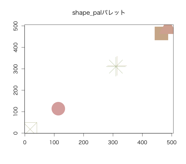
#shape_pal palette
#Automatically sets symbols for up to 6 groups; more than 6 will result in an error.
plot(TestData[, 2], TestData[, 2], pch = dscale(TestData[, 1], shape_pal(solid = TRUE)), cex = 6, xlab = "", ylab = "",
     main = "shape_pal palette", col = dscale(TestData[, 1], hue_pal(h = c(0, 160) + 15, c = 30, l = 75, h.start = 0, direction = 1)))