Analysis in R: managing plots in the browser. The “httpgd” package

This package allows plots to be managed in a browser or RStudio’s viewer. The operations that can be managed include saving plots in formats such as png and svg, zooming plots, etc.

Package version is 1.3.1. Checked with R version 4.2.2.

Install Package

Run the following command. Compilation is required during installation.

#Install Package
install.packages("httpgd")

Example

See the command and package help for details.

#Loading the library
library("httpgd")

#Preparing to display the plot in the browser: hgd command
#Works with your system's default browser
#Plots to be executed after this command are displayed
hgd()

#Viewing plots in default browser: hgd_browse command
hgd_browse()

#Viewing plots in RStudio: hgd_view command
hgd_view()

#Unlink the default browser: hgd_close command
hgd_close()

#Show httpgd_graphics_device information: hgd_info command
hgd_info(which = dev.cur())

#############################################
###Example: Viewed in a default browser######
#############################################
hgd()

###Creating Data#####
#Install the tidyverse package if it is not already present
if(!require("tidyverse", quietly = TRUE)){
  install.packages("tidyverse");require("tidyverse")
}
set.seed(1234)
n <- 300
TestData <- tibble(Group = sample(paste0("Group", 1:4), n,
                                  replace = TRUE),
                   X_num_Data = sample(c(1:50), n, replace = TRUE),
                   Y_num_Data = sample(c(51:100), n, replace = TRUE),
                   Chr_Data = sample(c("か", "ら", "だ", "に",
                                       "い", "い", "も", "の"),
                                     n, replace = TRUE),
                   Fct_Data = factor(sample(c("か", "ら", "だ", "に",
                                              "い", "い", "も", "の"),
                                            n, replace = TRUE)))
#######

#Install the GGally package if it is not already present
if(!require("GGally", quietly = TRUE)){
  install.packages("GGally");require("GGally")
}
#Plotting data features at once: GGally::ggpairs command
ggpairs(data = TestData, columns = c(1, 5, 2, 3),
        mapping = aes(color = Group),
        upper = list(continuous = "smooth"),
        lower = list(combo = "facetdensity"),
        diag = list(continuous = "barDiag"),
        cardinality_threshold = 30)

#Plotting multiple graphs: GGally:: command
PlotList <- list()
list(for (i in 1:3) {
  #Box plot
  PlotList[[i]] <- qplot(data = TestData, x = Group,
                         y = X_num_Data, fill = Group, geom = "boxplot")
  #Scatter plot
  PlotList[[i + 3]] <- qplot(data = TestData, x = Y_num_Data,
                             y = X_num_Data, color = Group, geom = "point") +
    ggtitle("TEST")
})

#Plot
ggmatrix(PlotList, nrow = 2, ncol = 3,
         xAxisLabels = 1:3, yAxisLabels = 1:2, title = "TEST")

#Create ggplot2 objyect
One_Cotinuous <- ggplot(TestData, aes(x = X_num_Data,
                                      color = Group,
                                      fill = Group))

#geom_area command
One_Cotinuous +
  geom_area(stat = "count", alpha = 0.7) +
  scale_fill_manual(values = c("#a87963", "#505457",
                               "#4b61ba", "#A9A9A9")) +
  labs(title = "geom_area")

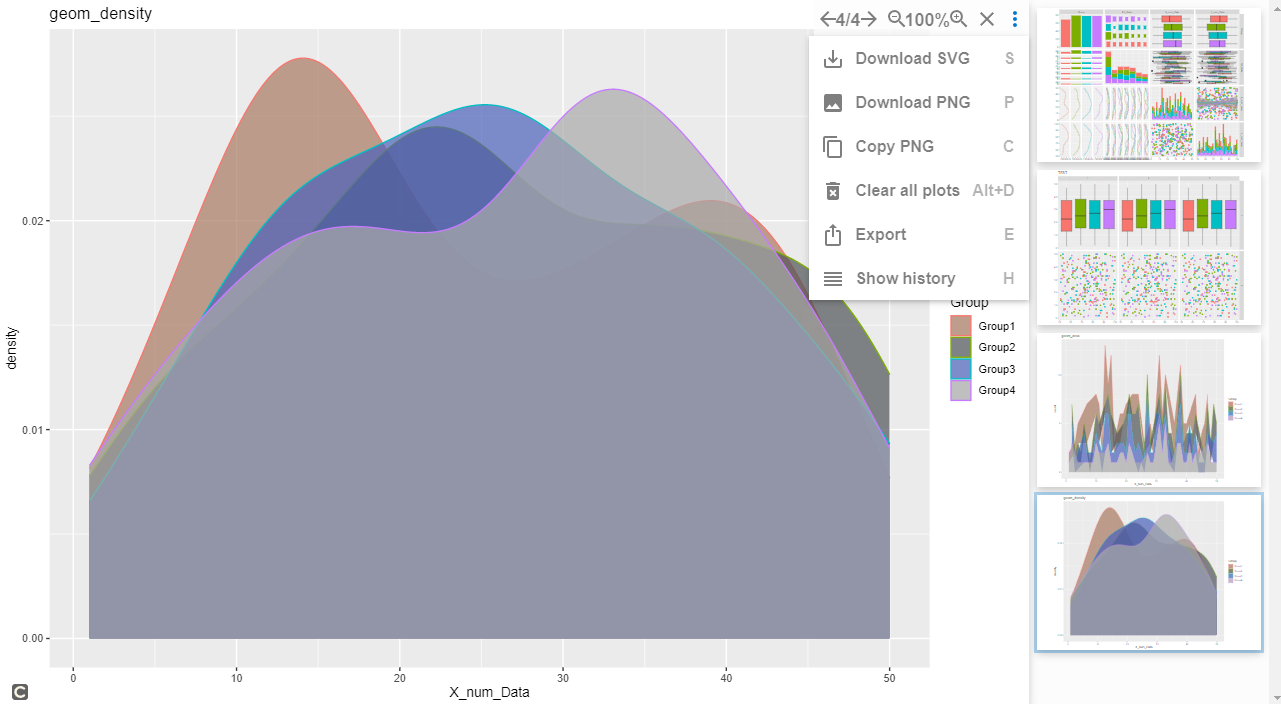
#geom_density command
One_Cotinuous +
  geom_density(alpha = 0.7) +
  scale_fill_manual(values = c("#a87963", "#505457",
                               "#4b61ba", "#A9A9A9")) +
  labs(title = "geom_density")

#Viewing plots in default browser: hgd_browse command
hgd_browse()
########

Output Example

I hope this makes your analysis a little easier !!