Smartwatches are increasingly used for health management and research. The “FITfileR” package is a convenient way to read data from Garmin, popular with marathon runners and others, in R.
Garmin works with Garmin Connect, which allows users to check various data on a smartphone app or website.
The data available on the Garmin Connect Web site is a binary file called a “fit file.
Flexible and Interoperable Data Transfer (FIT) SDK:https://developer.garmin.com/fit/overview/
The “fit file” protocol is available to the public, so those interested can analyze the file with the “readBin” command.
Note that, as introduced in Example, the time starting point of the “fit file” is “December 31, 1989 UTC (631065600)”, so “timestamp_16” uses 631065600 as the offset.
You may want to consider using a Garmin smartwatch for health management and research purposes. The Garmin I use is the VÍVOSMART 5. It can track a variety of health information such as sleep and stress.
Package version is 0.1.5. Checked with R version 4.2.2.
Get the fit file
Garmin and Garmin Connect are assumed to be paired. Please check the Garmin Web site and other sites for the connection method.
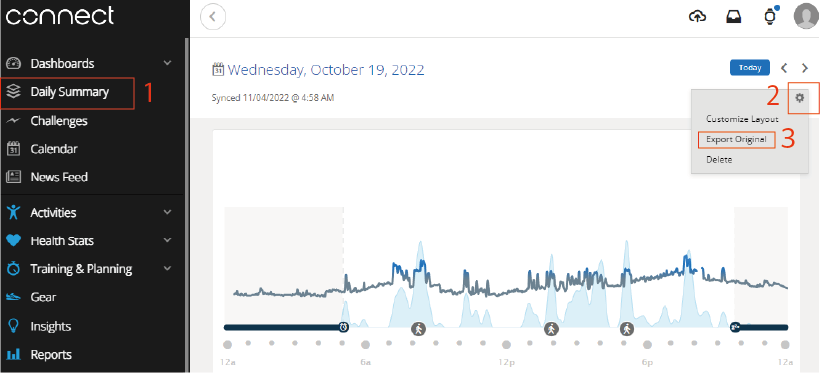
First, access Garmin Connect.
Garmin Connect:https://connect.garmin.com/signin/
After accessing the site, the fit file can be obtained by following the steps below. The “fit file” for any given day can be obtained as a zipped file.
Install Package
Run the following command.
#Install Package
if(!requireNamespace("remotes")) {
  install.packages("remotes")
}
remotes::install_github("grimbough/FITfileR")
Example
Refer to the commands and help for each package for details, and extract the zip file you received from Garmin Connect. The following is an example of a command that will process all WELLNESS.fit files in the extracted folder to obtain heart rate and stress level data. The “listMessageTypes” command can be used to check the target fit file for messages, and the “getMessagesByType” command can be used to get the target data.
#Loading the library
library("FITfileR")
#Install the tidyverse package if it is not already there
if(!require("tidyverse", quietly = TRUE)){
  install.packages("tidyverse");require("tidyverse")
}
#Install the lubridate package if it is not already there
#https://www.karada-good.net/analyticsr/r-467/
if(!require("lubridate", quietly = TRUE)){
  install.packages("lubridate");require("lubridate")
}

#Read fit files
#ReadFit <- readFitFile(file.choose())

#Check
#listMessageTypes(ReadFit)
#[1] "file_id"         "event"           "device_info"     "software"
#[5] "monitoring"      "monitoring_info" "ohr_settings"    "stress_level"

###Preparation for Continuous Processing#####
#Make the folder of the extracted fit file the working directory
setwd(choose.dir())

#Get file name
GetFileNames <- list.files()

#Target "XXX_WELLNESS.fit"
AnaFileNames <- str_subset(GetFileNames, "WELLNESS")

#Arguments for storing data
ActivityData <- NULL
HartRateData <- NULL
StressData <- NULL

###Iterative processing#####
for(i in seq(AnaFileNames)){

  ReadFit <- readFitFile(AnaFileNames[[i]])

  if("event" %in% listMessageTypes(ReadFit)){
###Activity and Heart Rate acquisition#####
MonitoringData <- getMessagesByType(ReadFit,
                                    message_type = "monitoring")

#Batch conversion of dates
for(n in seq(MonitoringData)){

  #conversion of dates
  MonitoringData[[n]] <-
    MonitoringData[[n]] %>%
    mutate_if(is.POSIXt, ~with_tz(., tz = "America/New_York"))

}

###Conversion of timestamp_16#####
#Reference:https://developer.garmin.com/fit/cookbook/datetime/
#The time starting point of the fit file is "December 31, 1989 UTC (631065600)",
#so "timestamp_16" uses 631065600 as the offset.
#Get "fit" file start time
TimCre <- as.numeric(as.POSIXct(file_id(ReadFit)[[2]])[[1]]) - 631065600

#Conversion process
for(n in seq(MonitoringData)){

  #Conversion of Date Data
  MonitoringData[[n]] <-
    MonitoringData[[n]] %>%
    mutate_at(vars(matches("timestamp_16")),
              function(.){
                TimCre +
                  bitwAnd((. - TimCre), 0xffff) + 631065600 %>%
                  lubridate::as_datetime() %>%
                  lubridate::with_tz(tz = "Asia/Tokyo")})
}
########

###Get activity data#####
#Get list number of column names containing "current_activity_type_intensity"
ActivityNo <- which(sapply(MonitoringData,
                           function(x) "current_activity_type_intensity" %in% colnames(x)))

for(For_ActiNo in seq(length(ActivityNo))){
if("timestamp" %in% colnames(MonitoringData[[ActivityNo[For_ActiNo]]])){

  ActivityData <- bind_rows(ActivityData,
                            MonitoringData[[ActivityNo[For_ActiNo]]])

}else{

  MonitoringData[[ActivityNo[For_ActiNo]]] %>%
    select("timestamp_16", "current_activity_type_intensity") %>%
    bind_rows(ActivityData)

}}

###Get heart rate data#####
#Get list number of column names containing "heart_rate"
HartRateNo <- which(sapply(MonitoringData, function(x) "heart_rate" %in% colnames(x)))
#HartRate <- rbind(HartRate, MonitoringData[[HartRateNo]])
HartRateData <- bind_rows(HartRateData, MonitoringData[[HartRateNo]])

###Get stress levels#####
StressLevelData <- getMessagesByType(ReadFit,
                                     message_type = "stress_level") %>%
  mutate_if(is.POSIXt, ~with_tz(., tz = "Asia/Tokyo"))

#StressData <- rbind(StressData, StressLevelData)
StressData <- bind_rows(StressData, StressLevelData)

  }
}

#Prepare column names
colnames(ActivityData) <- c("Time_Stamp", "Activity_type_intensity")
colnames(HartRateData) <- c("Time_Stamp", "Hart_Rate")
colnames(StressData) <- c("Time_Stamp", "Stress_Level")

#Delete all data except "ActivityData", "HartRate", and "StressData
remove(list = ls()[!ls() %in% c("ActivityData", "HartRateData", "StressData")])
########
Output Example
・Plot heart rate data
#Install the tidyverse package if it is not already there
if(!require("tidyverse", quietly = TRUE)){
  install.packages("tidyverse");require("tidyverse")
}
ggplot(HartRateData, aes(x = Time_Stamp, y = Hart_Rate)) +
  geom_area(fill = "#4b61ba") +
  labs(title = "Hart_Rate") +
  theme_minimal()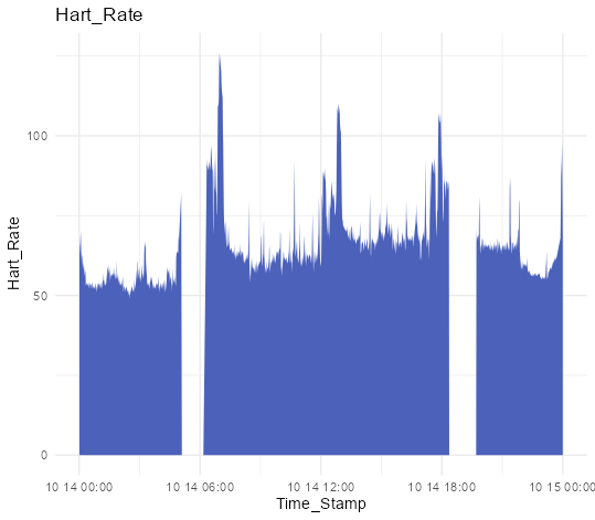
・Plot Stress Data
#Install the tidyverse package if it is not already there
if(!require("tidyverse", quietly = TRUE)){
  install.packages("tidyverse");require("tidyverse")
}
ggplot(StressData, aes(x = Time_Stamp, y = Stress_Level)) +
geom_area(fill = "#a87963") +
labs(title = "Stress_Level") +
theme_minimal()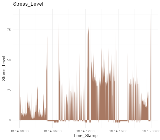
I hope this makes your analysis a little easier !!