Analysis in R: Representing data features as circles. The “packcircles” package

This is an introduction to a package that displays the characteristics of data as a circle. Note that the graphing is done in conjunction with the “ggplot2” package. The Example command also presents an example of creating an interactive graph in conjunction with the “ggiraph” package.

Package version is 0.3.4. Checked with R version 4.2.2.

Install Package

Run the following command.

#Install Package
install.packages("packcircles")

Example

See the command and package help for details.

#Loading the library
library("packcircles")

###Creating Data#####
#Install the tidyverse package if it is not already there
if(!require("tidyverse", quietly = TRUE)){
  install.packages("tidyverse");require("tidyverse")
}
n <- 300
TestData1 <- data.frame(Value = 1:n,
                           id = 1:n,
                           Name = sample(LETTERS[1:24], n, replace = TRUE)) %>%
  mutate(Col = if_else(Value %% 2 == 0, "#9e323a", "#7edbf2"))
TestData2 <- data.frame(Value = n:1,
                           id = 1:n,
                           Name = sample(LETTERS[1:24], n, replace = TRUE)) %>%
  mutate(Col = if_else(Value %% 2 == 0, "#df6d68", "#f6adad"))
########

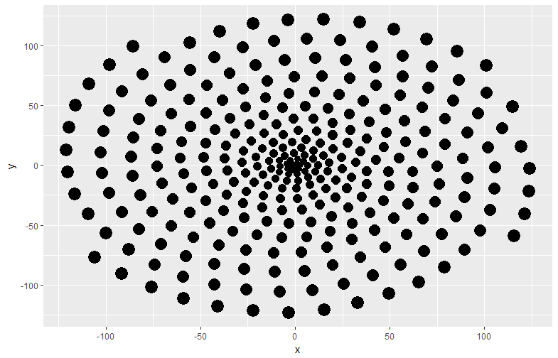
#Create a layout that avoids overlapping circles: circleProgressiveLayout command
#Specify circle size data: sizecol option
#How to specify size: sizetype option; choose from "area", "radius
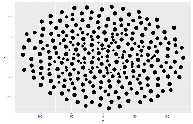
CPData <- circleProgressiveLayout(TestData1, sizecol = 1, sizetype = "area")
ggplot(data = CPData, aes(x, y, size = radius)) +
  geom_point(col = "black", show.legend = FALSE)

#Create a non-overlapping layout using iterative pairwise: circleRepelLayout command
#If data is not in center x, center y, radius order
#Set xysizecols option to c(NA, NA, 1)
#Specify number of iterations: maxiter option; the higher the number, the better the accuracy
CRData <- circleRepelLayout(TestData1, xysizecols = c(NA, NA, 1),
                               sizetype = "area", maxiter = 1500)
ggplot(data = CRData$layout, aes(x, y, size = radius)) +
  geom_point(col = "black", show.legend = FALSE)

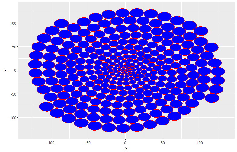
#Converted to the format used by ggplot2: circleLayoutVertices command
#Can use geom_polygon command
GGCPData <- circleLayoutVertices(CPData)
ggplot(data = GGCPData, aes(x, y, group = id)) +
  geom_polygon(col = "red", fill = "blue", show.legend = FALSE)

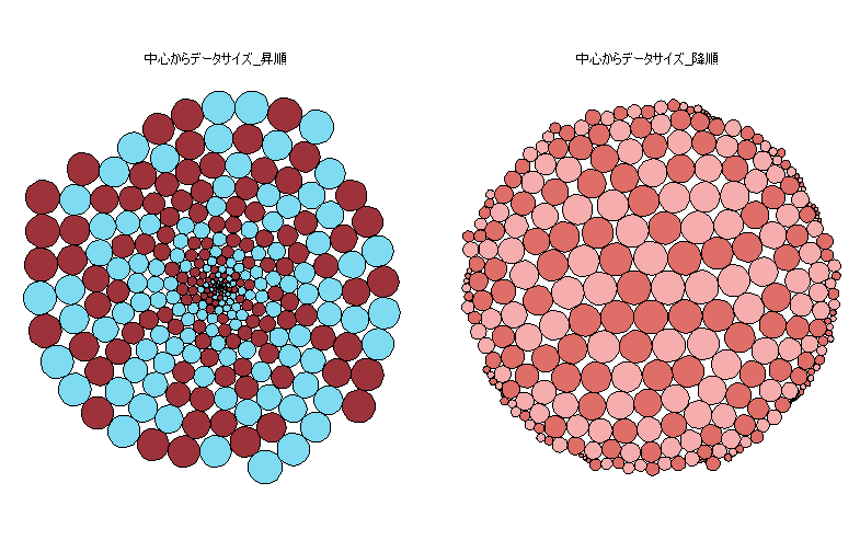
###Example: Interactive graph#####
#install.packages("ggiraph")
library("ggiraph")
#Data from center ascending
GetLayout1 <- circleProgressiveLayout(TestData1, sizecol = 1, sizetype = "radius") 
TestPlotData1 <- circleLayoutVertices(GetLayout1) %>%
  left_join(TestData1[, c(2, 3:4)], by = "id")
#Data from center descending
GetLayout2 <- circleProgressiveLayout(TestData2, sizecol = 1, sizetype = "radius") 
TestPlotData2 <- circleLayoutVertices(GetLayout2) %>%
  left_join(TestData2[, c(2, 3:4)], by = "id")
#Combine data to adapt facet
PlotData <- rbind(cbind(TestPlotData1, set = 1),
                     cbind(TestPlotData2, set = 2) )
#Plot Preparation
IntGg <- ggplot(data = PlotData, aes(x, y, group = id)) +
  geom_polygon_interactive(fill = PlotData$Col, col = "black",
                           tooltip = PlotData$Name, show.legend = FALSE) +
  facet_wrap(~ set, labeller = as_labeller(c("1" = "ascending",
                                             "2" = "descending"))) +
  theme_void() +
  coord_equal()
#Plot
ggiraph(ggobj = IntGg, width_svg = 5,
        height_svg = 3, zoom_max = 10)