This is a quick summary of how to specify col and fill colors in ggplot2, which is often forgotten. I think it will be easier to understand if you are aware of the discrete and continuous values set on the axes.
tidyverse package version is 1.3.1. Checked with R version 4.2.2.
Install Package
Run the following command.
#Install Package
#install.packages("ggplot2")
install.packages("tidyverse")
Summary of color specification methods
See the command and package help for details.
#Loading the library
#library("ggplot2")
library("tidyverse")
###Preparations#####
#Creating Data
n <- 300
PlotData <- data.frame(ID = rep(1:5, len = n),
Group = sample(c("A", "B", "C"), n, replace = TRUE),
Time_A = abs(rnorm(n)), Time_B = -log2(abs(rnorm(n))))
#Assign color with Group datas
PlotData <- PlotData %>%
#case_when command is specified by conditional expression ~ result
mutate(GroupCol = case_when(Group == "A" ~ "#a0b981",
Group == "B" ~ "#47547c",
Group == "C" ~ "#9f8288"))
#Check Color
#https://www.karada-good.net/analyticsr/r-109
#install.packages("scales")
#library("scales")
#show_col(c("#a0b981", "#47547c", "#9f8288"))
#Package useful for displaying plots side by side
#https://www.karada-good.net/analyticsr/r-591
#install.packages("multipanelfigure")
library("multipanelfigure")
########
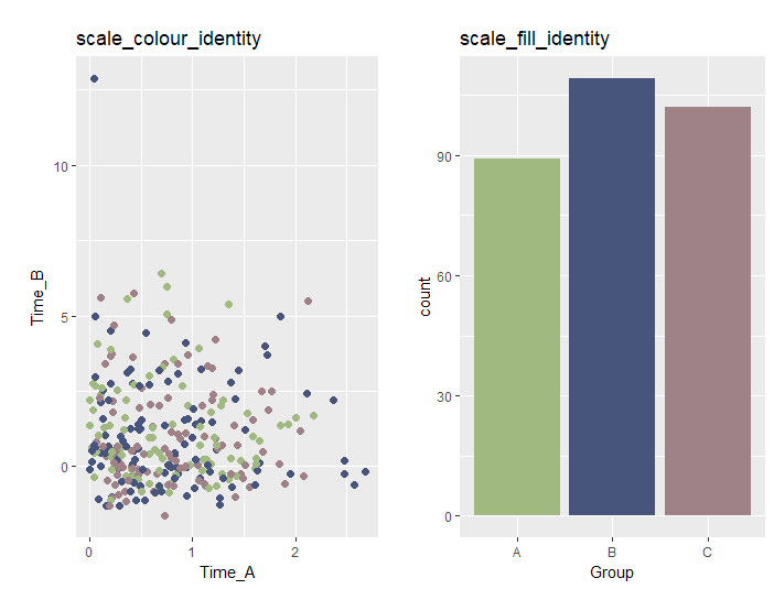
###If the data contains color datas: "scale_XXX_identity" command#####
#If you specify col: "scale_color_identity" command
PointPlot <- ggplot(PlotData, aes(x = Time_A, y = Time_B)) +
geom_point(aes(col = GroupCol), size = 2) +
scale_colour_identity(guide = "none") +
labs(title = "scale_colour_identity")
#If you specify fill: "scale_fill_identity" command
BarPlot <- ggplot(PlotData, aes(x = Group)) +
geom_bar(aes(fill = GroupCol)) +
scale_fill_identity(guide = "none") +
labs(title = "scale_fill_identity")
#Plot
multi_panel_figure(columns = 2, rows = 1) %>%
fill_panel(panel = PointPlot, column = 1, row = 1, label = "") %>%
fill_panel(panel = BarPlot, column = 2, row = 1, label = "")
########
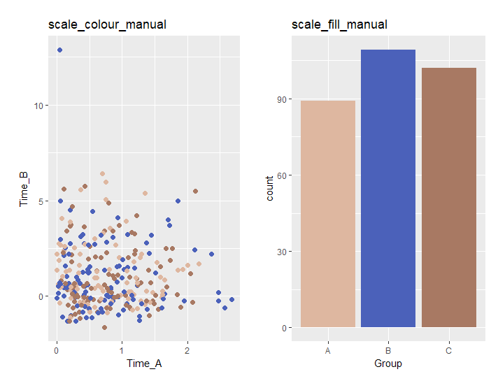
###If the data contains color datas: scall_XXX_manual command#####
#If you specify col: "scale_colour_manual" command
PointPlot <- ggplot(PlotData, aes(x = Time_A, y = Time_B)) +
geom_point(aes(col = Group), size = 2) +
scale_colour_manual(values = c("#deb7a0", "#4b61ba", "#a87963"), guide = "none") +
labs(title = "scale_colour_manual")
#If you specify fill: "scale_fill_manual" command
BarPlot <- ggplot(PlotData, aes(x = Group)) +
geom_bar(aes(fill = Group)) +
scale_fill_manual(values = c("#deb7a0", "#4b61ba", "#a87963"), guide = "none") +
labs(title = "scale_fill_manual")
#Plot
multi_panel_figure(columns = 2, rows = 1) %>%
fill_panel(panel = PointPlot, column = 1, row = 1, label = "") %>%
fill_panel(panel = BarPlot, column = 2, row = 1, label = "")
#######
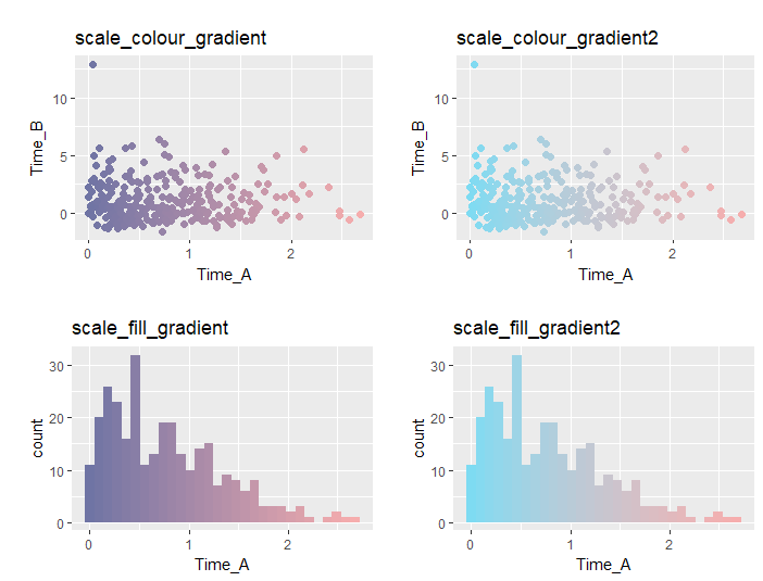
###Gradienting: scall_XXX_gradient,scall_XXX_gradient2 command#####
#If you specify col: scale_colour_gradient command
#The data specified for col is a continuous variable
PointPlot1 <- ggplot(PlotData, aes(x = Time_A, y = Time_B)) +
geom_point(aes(col = Time_A), size = 2) +
scale_colour_gradient(low = "#6f74a4", high = "#f6adad", guide = "none") +
labs(title = "scale_colour_gradient")
#If you specify col: scale_colour_gradient2 command#
#The data specified for col is a continuous variable
PointPlot2 <- ggplot(PlotData, aes(x = Time_A, y = Time_B)) +
geom_point(aes(col = Time_A), size = 2) +
scale_colour_gradient2(low = "#6f74a4", high = "#f6adad", mid = "#7edbf2", guide = "none") +
labs(title = "scale_colour_gradient2")
#If you specify fill: "scale_fill_gradient" command
histogram1 <- ggplot(PlotData, aes(x = Time_A)) +
geom_histogram(aes(fill = ..x..)) +
scale_fill_gradient(low = "#6f74a4", high = "#f6adad", guide = "none") +
labs(title = "scale_fill_gradient")
#If you specify fill: "scale_fill_gradient2" command
histogram2 <- ggplot(PlotData, aes(x = Time_A)) +
geom_histogram(aes(fill = ..x..)) +
scale_fill_gradient2(low = "#6f74a4", high = "#f6adad", mid = "#7edbf2", guide = "none") +
labs(title = "scale_fill_gradient2")
#Plot
multi_panel_figure(columns = 2, rows = 2) %>%
fill_panel(panel = PointPlot1, column = 1, row = 1, label = "") %>%
fill_panel(panel = PointPlot2, column = 2, row = 1, label = "") %>%
fill_panel(panel = histogram1, column = 1, row = 2, label = "") %>%
fill_panel(panel = histogram2, column = 2, row = 2, label = "")
########
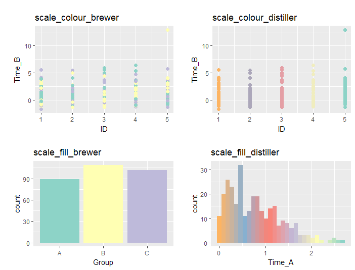
###Use color palette: scall_XXX_brewer,scall_XXX_distiller commands#####
#Check the color palette with
#the following command:RColorBrewer::display.brewer.all()
#If you specify col: "scale_colour_brewer" command
PointPlot1 <- ggplot(PlotData, aes(x = ID, y = Time_B)) +
geom_point(aes(col = Group), size = 2) +
scale_colour_brewer(palette = "Set3", guide = "none") +
labs(title = "scale_colour_brewer")
#If you specify col: scale_colour_distiller command
PointPlot2 <- ggplot(PlotData, aes(x = ID, y = Time_B)) +
geom_point(aes(col = ..x..), size = 2) +
scale_colour_distiller(palette = "Set3", guide = "none") +
labs(title = "scale_colour_distiller")
#If you specify fill: "scale_fill_brewer" command
histogram1 <- ggplot(PlotData, aes(x = Group)) +
geom_histogram(aes(fill = Group), stat="count") +
scale_fill_brewer(palette = "Set3", guide = "none") +
labs(title = "scale_fill_brewer")
#If you specify fill: scale_fill_distiller command
histogram2 <- ggplot(PlotData, aes(x = Time_A)) +
geom_histogram(aes(fill = ..x..)) +
scale_fill_distiller(palette = "Set3", guide = "none") +
labs(title = "scale_fill_distiller")
#Plot
multi_panel_figure(columns = 2, rows = 2) %>%
fill_panel(panel = PointPlot1, column = 1, row = 1, label = "") %>%
fill_panel(panel = PointPlot2, column = 2, row = 1, label = "") %>%
fill_panel(panel = histogram1, column = 1, row = 2, label = "") %>%
fill_panel(panel = histogram2, column = 2, row = 2, label = "")
########
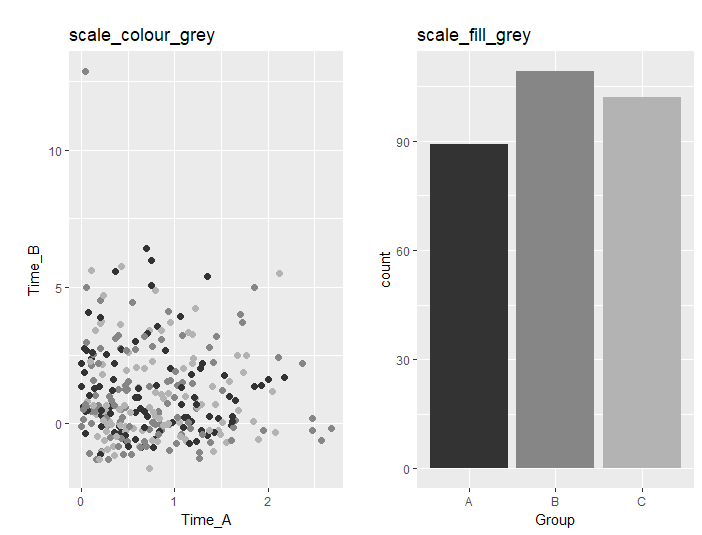
###Grayscaling: scale_XXX_grey command#####
#If you specify col: "scale_colour_grey" command
PointPlot <- ggplot(PlotData, aes(x = Time_A, y = Time_B)) +
geom_point(aes(col = Group), size = 2) +
scale_colour_grey(start = .2, end = .7, guide = "none") +
labs(title = "scale_colour_grey")
#If you specify fill:"scale_fill_grey" command
BarPlot <- ggplot(PlotData, aes(x = Group)) +
geom_bar(aes(fill = Group)) +
scale_fill_grey(start = .2, end = .7, guide = "none") +
labs(title = "scale_fill_grey")
#Plot
multi_panel_figure(columns = 2, rows = 1) %>%
fill_panel(panel = PointPlot, column = 1, row = 1, label = "") %>%
fill_panel(panel = BarPlot, column = 2, row = 1, label = "")
########Output Example
If the data contains color datas
・scale_XXX_identity command
Specify color data
・scall_XXX_manual command
Gradienting
・scall_XXX_gradient,scall_XXX_gradient2 command
Use color palette
・scall_XXX_brewer,scall_XXX_distiller command
Grayscaling
・scale_XXX_grey command
I hope this makes your analysis a little easier !!