The following are examples of plots in the “ggplot2” package with “one variable: continuous variable” and “two variables: combination of continuous and discrete variables”. The commands for each data example are also presented, so please refer to the data format for the plots.
In order to use the “ggplot2” package, the “tidyverse” package is used.
Package version is 1.3.1. Checked with R version 4.2.2.
Install Package
Run the following command.
#Install Package
install.packages("tidyverse")
Example
・Loading the “tidyverse” package and creating example data
#Loading the library
library("tidyverse")
###Creating Data#####
set.seed(1234)
n <- 300
TestData <- tibble(Group = sample(paste0("Group", 1:4), n,
replace = TRUE),
X_num_Data = sample(c(1:50), n, replace = TRUE),
Y_num_Data = sample(c(51:100), n, replace = TRUE),
Chr_Data = sample(c("か", "ら", "だ", "に",
"い", "い", "も", "の"),
n, replace = TRUE),
Fct_Data = factor(sample(c("か", "ら", "だ", "に",
"い", "い", "も", "の"),
n, replace = TRUE)))
#Check
TestData
# A tibble: 300 x 5
Group X_num_Data Y_num_Data Chr_Data Fct_Data
<chr> <int> <int> <chr> <fct>
1 Group4 31 83 だ い
2 Group4 33 95 か に
3 Group2 45 74 ら い
4 Group2 10 99 い い
5 Group1 22 90 の だ
6 Group4 13 65 い に
7 Group3 27 76 い ら
8 Group1 40 66 だ ら
9 Group1 18 92 い も
10 Group2 23 84 の も
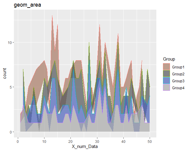
#######・One variable: plots that can be created with continuous variables
#Creation of basic ggplot2 plot
One_Cotinuous <- ggplot(TestData, aes(x = X_num_Data,
color = Group,
fill = Group))
#geom_area command
#Set the aggregation method: stat option; "bin", "count", "density", etc.
One_Cotinuous +
geom_area(stat = "count", alpha = 0.7) +
scale_fill_manual(values = c("#a87963", "#505457",
"#4b61ba", "#A9A9A9")) +
labs(title = "geom_area")
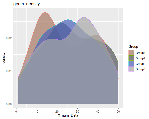
#geom_density command
One_Cotinuous +
geom_density(alpha = 0.7) +
scale_fill_manual(values = c("#a87963", "#505457",
"#4b61ba", "#A9A9A9")) +
labs(title = "geom_density")
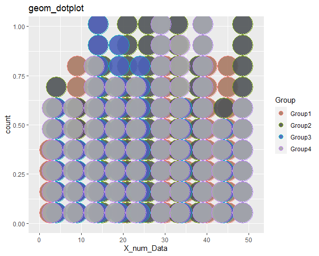
#geom_dotplot command
#Bin display method: method options; "dotdensity", "histodot"
One_Cotinuous +
geom_dotplot(method = "dotdensity", binwidth = 5, alpha = 0.9) +
scale_fill_manual(values = c("#a87963", "#505457",
"#4b61ba", "#A9A9A9")) +
labs(title = "geom_dotplot")
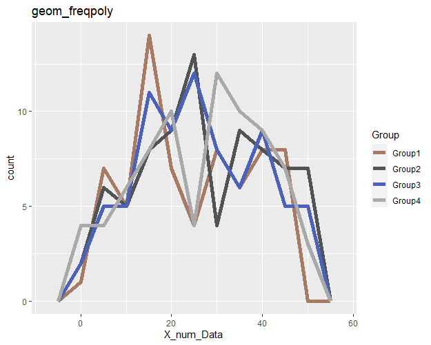
#geom_freqpoly command
One_Cotinuous +
geom_freqpoly(binwidth = 5, size = 2) +
scale_color_manual(values = c("#a87963", "#505457",
"#4b61ba", "#A9A9A9")) +
labs(title = "geom_freqpoly")
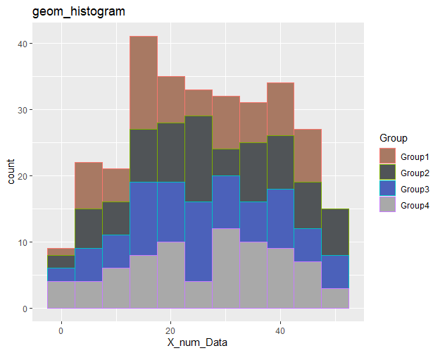
#geom_histogram command
One_Cotinuous +
geom_histogram(binwidth = 5) +
scale_fill_manual(values = c("#a87963", "#505457",
"#4b61ba", "#A9A9A9")) +
labs(title = "geom_histogram")
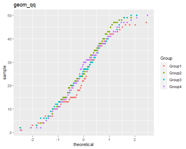
#geom_qq command
ggplot(TestData) +
geom_qq(aes(sample = X_num_Data, colour = Group)) +
scale_fill_manual(values = c("#a87963", "#505457",
"#4b61ba", "#A9A9A9")) +
labs(title = "geom_qq")
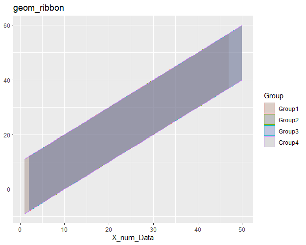
#geom_ribbon command
One_Cotinuous +
geom_ribbon(aes(ymin = X_num_Data - 10, ymax = X_num_Data + 10),
alpha = 0.3) +
scale_fill_manual(values = c("#a87963", "#505457",
"#4b61ba", "#A9A9A9")) +
labs(title = "geom_ribbon")【Output Example】
・Two variables: x and y both continuous variables Plots that can be created with
#Creation of basic ggplot2 plot
Two_Cotinuous <- ggplot(TestData, aes(x = X_num_Data,
y = Y_num_Data,
color = Group,
fill = Group))
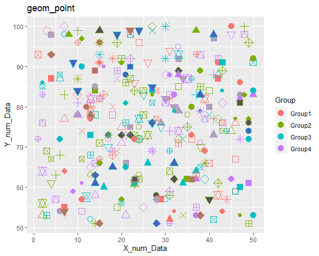
#geom_point command
#Specify symbol: shape option; up to 0:25 can be specified
#All types of plots in the example
Two_Cotinuous +
geom_point(alpha = 1, size = 4, shape = rep(0:25, length = 300)) +
scale_fill_manual(values = c("#a87963", "#505457",
"#4b61ba", "#A9A9A9")) +
labs(title = "geom_point")
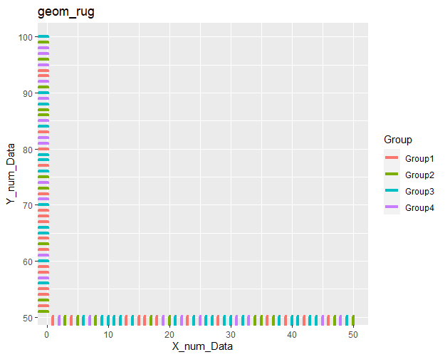
#geom_rug command
Two_Cotinuous +
geom_rug(size = 1.5) +
scale_fill_manual(values = c("#a87963", "#505457",
"#4b61ba", "#A9A9A9")) +
labs(title = "geom_rug")
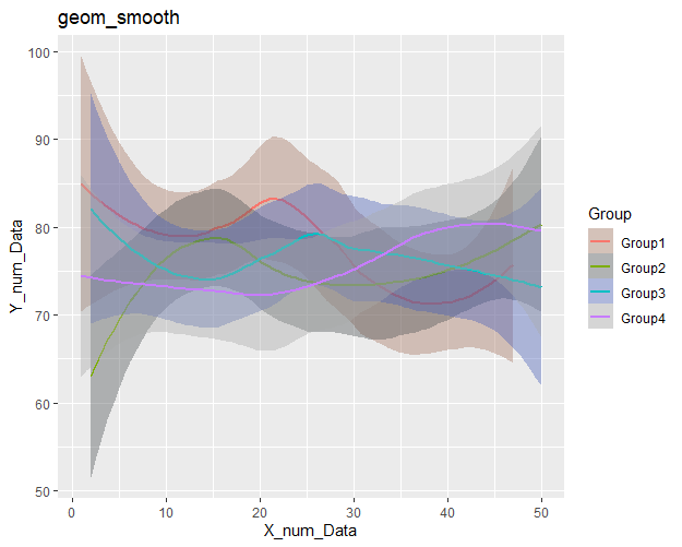
#geom_smooth command
Two_Cotinuous +
geom_smooth() +
scale_fill_manual(values = c("#a87963", "#505457",
"#4b61ba", "#A9A9A9")) +
labs(title = "geom_smooth")
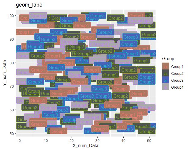
#geom_label command
Two_Cotinuous +
geom_label(aes(label = Group)) +
scale_fill_manual(values = c("#a87963", "#505457",
"#4b61ba", "#A9A9A9")) +
labs(title = "geom_label")
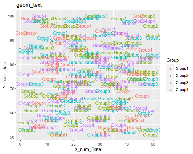
#geom_text command
Two_Cotinuous +
geom_text(aes(label = Group)) +
scale_fill_manual(values = c("#a87963", "#505457",
"#4b61ba", "#A9A9A9")) +
labs(title = "geom_text")【Output Example】
・Two variables: discrete variables, plots that can be created by combining continuous variables
#Creation of basic ggplot2 plot
#Use up to 100 data to make plots easier to read
Discrete_Cotinuous <- ggplot(TestData[1:100,],
aes(x = Group, y = X_num_Data,
color = Group, fill = Group))
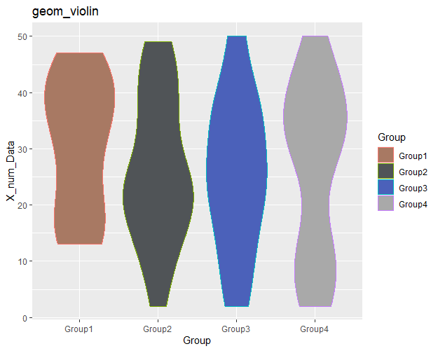
#geom_violin command
Discrete_Cotinuous +
geom_violin() +
scale_fill_manual(values = c("#a87963", "#505457",
"#4b61ba", "#A9A9A9")) +
labs(title = "geom_violin")
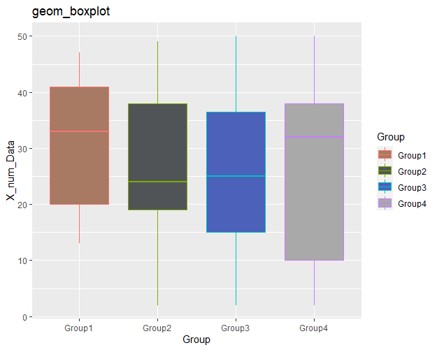
#geom_boxplot command
Discrete_Cotinuous +
geom_boxplot() +
scale_fill_manual(values = c("#a87963", "#505457",
"#4b61ba", "#A9A9A9")) +
labs(title = "geom_boxplot")
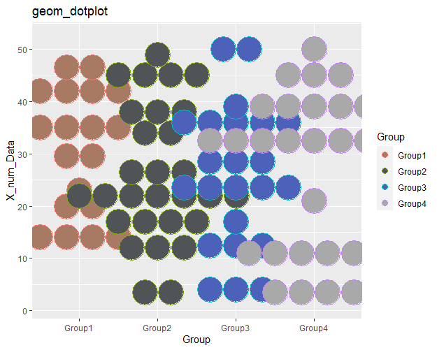
#geom_dotplot command
#Display dots: stackdir option; "up","down","center","centerwhole"
Discrete_Cotinuous +
geom_dotplot(binaxis = "y", stackdir = "center", binwidth = 5) +
scale_fill_manual(values = c("#a87963", "#505457",
"#4b61ba", "#A9A9A9")) +
labs(title = "geom_dotplot")
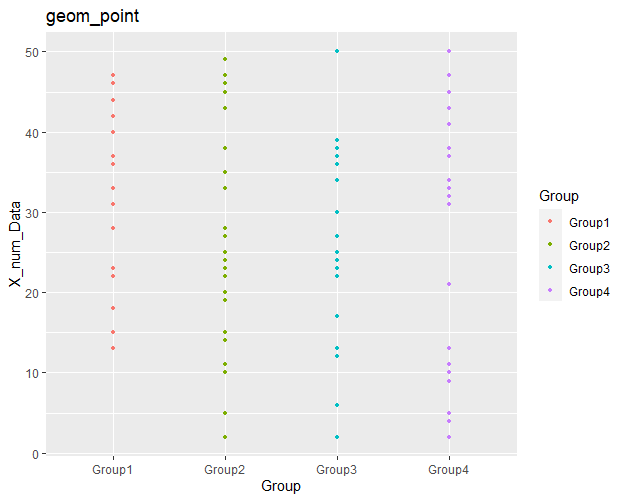
#geom_point command
Discrete_Cotinuous +
geom_point(size = 1) +
scale_fill_manual(values = c("#a87963", "#505457",
"#4b61ba", "#A9A9A9")) +
labs(title = "geom_point")【Output Example】
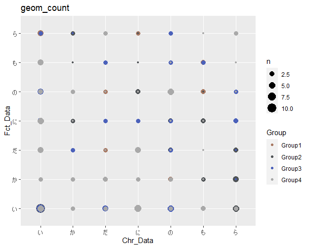
・Two variables: plots that can be created by combining discrete variables for both x and y
#Creation of basic ggplot2 plot
Two_Discrete <- ggplot(TestData, aes(x = Chr_Data,
y = Fct_Data,
color = Group,
fill = Group))
#geom_count command
Two_Discrete +
geom_count() +
scale_color_manual(values = c("#a87963", "#505457",
"#4b61ba", "#A9A9A9")) +
labs(title = "geom_count")
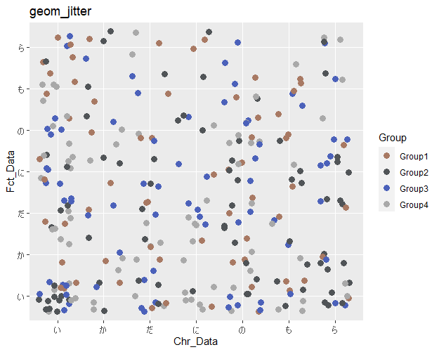
#geom_jitter command
Two_Discrete +
geom_jitter(size = 3) +
scale_color_manual(values = c("#a87963", "#505457",
"#4b61ba", "#A9A9A9")) +
labs(title = "geom_jitter")【Output Example】
I hope this makes your analysis a little easier !!