Introducing the “missRanger” package for assigning missing values in a chained random forest. This package is useful for creating and assigning missing values.
Package version is 2.2.0. Checked with R version 4.2.2.
Install Package
Run the following command.
#Install Package
install.packages("missRanger")
Example
See the command and package help for details.
#Loading the library
library("missRanger")
###Create Data#####
set.seed(1234)
n <- 10
TestData <- data.frame(Group = sample(paste0("Group ", 1:2), n, replace = TRUE),
Time_1 = round(rnorm(n) - 1.5, 2),
Time_2 = round(rnorm(n), 2),
Time_3 = round(rnorm(n) - 1.5, 2))
TestData[1:4, 2:4] <- sample(1:2, 12, replace = TRUE)
########
#Assign missing values to data: generateNA command
#Specify data: x option; vector, matrix, data.frame can be specified
#Probability to assign missing values per column: p option; range 0.1-1.0
#Set seed: seed option
ResultData <- generateNA(x = TestData, p = 0.3, seed = 1234)
#Result
ResultData
# Group Time_1 Time_2 Time_3
#1 Group 2 2.00 2.00 2.00
#2 Group 2 1.00 NA 1.00
#3 Group 2 1.00 2.00 1.00
#4 Group 2 1.00 NA 2.00
#5 <NA> NA 2.42 -2.44
#6 <NA> NA 0.13 NA
#7 Group 1 -2.50 NA NA
#8 Group 1 -2.28 -0.44 -2.21
#9 Group 1 NA 0.46 -2.00
#10 <NA> -0.54 -0.69 NA
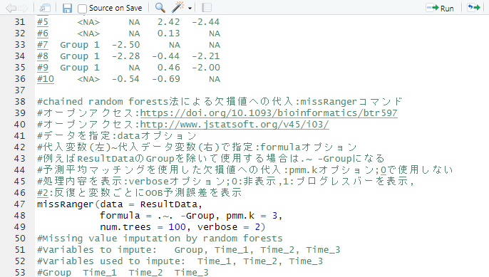
#Missing value assignment by chained random forest method: missRanger command
#Open access:https://doi.org/10.1093/bioinformatics/btr597
#Open access:http://www.jstatsoft.org/v45/i03/
#Specify data:data option
#Specify by assignment variable (left)~assigned data variable (right): formula option
#For example, to use ResultData without Group, use . ~ group
#Assign missing values using predictive mean matching: pmm.k option; not used with 0
#Display the process: verbose option;0:hide,1:show progress bar,.
#2:show OOB prediction error per iteration and variable
missRanger(data = ResultData,
formula = .~. -Group, pmm.k = 3,
num.trees = 100, verbose = 2)
#Missing value imputation by random forests
#Variables to impute: Group, Time_1, Time_2, Time_3
#Variables used to impute: Time_1, Time_2, Time_3
#Group Time_1 Time_2 Time_3
#iter 1: 1.0000 1.0000 0.9862 1.6359
#
# Group Time_1 Time_2 Time_3
#1 Group 2 2.00 2.00 2.00
#2 Group 2 1.00 2.42 1.00
#3 Group 2 1.00 2.00 1.00
#4 Group 2 1.00 -0.69 2.00
#5 Group 2 2.00 2.42 -2.44
#6 Group 2 2.00 0.13 1.00
#7 Group 1 -2.50 -0.44 2.00
#8 Group 1 -2.28 -0.44 -2.21
#9 Group 1 1.00 0.46 -2.00
#10 Group 2 -0.54 -0.69 -2.21I hope this makes your analysis a little easier !!