スパイラルチャートを手軽に作成できるパッケージの紹介です。よく使いそうなコマンドと気象庁からダウンロードできる札幌の気温データを使用した例を紹介します。
スパイラルチャートはアルキメデスの螺旋に沿ってプロットし表現する手法で、大規模なデータを視認するのに便利です。Spiral PlotやSpiral chartsで検索していただくと多くの情報を得ることが可能です。
パッケージバージョンは1.0.4。windows11のR version 4.1.2で確認しています。
パッケージのインストール
下記、コマンドを実行してください。
#パッケージのインストール
install.packages("spiralize")
実行コマンド
詳細はコメント、コマンドヘルプを確認してください。
###基本的な設定#####
#スパイラルチャートの設定:spiral_initializeコマンド
#チャートの開始点:startオプション
#チャートの終了点:endオプション
#start,endオプションは[360x + b]で直感的に設定できます
#反転の設定:flipオプション;"none","horizontal","vertical","both"
#データスケーリング設定:scale_byオプション
###"angle":極座標からの角度の差が等しくする
###"curve":スパイラルチャートにデータが収まるようにする
#データ軸の方向を設定:reverseオプション;TRUE,FALSE
#x軸範囲を指定:xlimオプション;c(min, max)
spiral_initialize(start = 360*1 + 0, end = 360*3 + 180,
flip = "none", scale_by = "angle",
reverse = FALSE, xlim = sRange)
#スパイラルチャートのトラック設定:spiral_trackコマンド
#トラックの幅を設定:heightオプション;0:1の範囲
#y軸範囲を指定:reverse_yオプション;c(min, max)
#データ軸の方向を設定:reverse_yオプション;TRUE,FALSE
#トラックの枠,塗色:background_gpオプション;gparコマンドで指定
spiral_track(height = 0.4, ylim = c(0, 1),
background_gp = gpar(col = "green", fill = 2))
#トラックは重ねることができます
spiral_track(height = 0.4, ylim = c(0, 1),
background_gp = gpar(col = "red", fill = "yellow"))
#x軸の設定:spiral_axisコマンド
#ラベルの位置:hオプション;"top","bottom"
#ラベルをカーブで曲げる:curved_labelsオプション;TRUE,FALSE
#フォントサイズを設定:labels_gpオプション;gparコマンドで指定
spiral_axis(h = "top", curved_labels = TRUE,
labels_gp = gpar(fontsize = 7))
#y軸の設定:spiral_yaxisコマンド
#ラベルの位置:sideオプション;"both","start","end"
spiral_yaxis(side = "both")
###参考#####
#スパイラルチャートのトラック数を確認:n_tracksコマンド
n_tracks()
[1] 2
#アクティブなスパイラルチャートのトラックを変更:set_current_trackコマンド
#スパイラルトラックを指定:track_index
set_current_track(track_index = 2)
#現在のアクティブなスパイラルチャートのトラック確認:current_track_indexコマンド
current_track_index()
[1] 2
########各種スパイラルチャート例
詳細はコメント、コマンドヘルプを確認してください。
###各種スパイラルチャート例#####
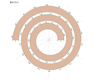
#各種スパイラルチャート例で使う基本プロットを作成
BasePlot <- function(){
#スパイラルチャートの設定
spiral_initialize(start = 360*1 + 0, end = 360*3 + 180,
flip = "none", scale_by = "angle",
reverse = FALSE, xlim = sRange)
#スパイラルチャートのトラック設定
spiral_track(height = 0.7, ylim = c(0, 1),
background_gp = gpar(col = "#426617", fill = "#deb7a0"))
#x軸の設定
spiral_axis(h = "top", curved_labels = TRUE,
labels_gp = gpar(fontsize = 7))
#y軸の設定
spiral_yaxis(side = "both")
}
#確認
BasePlot()
#スパイラルチャートタイトル
grid.text("基本プロット", x = 0, y = 1, just = c("left", "top"))
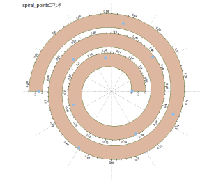
#散布図の描写:spiral_pointsコマンド
BasePlot()
spiral_points(x = seq(max, min, length = 10), y = ValueRunif,
pch = 16, gp = gpar(cex = 2, col = "#94bbe3"))
#スパイラルチャートタイトル
grid.text("spiral_pointsコマンド", x = 0, y = 1, just = c("left", "top"))
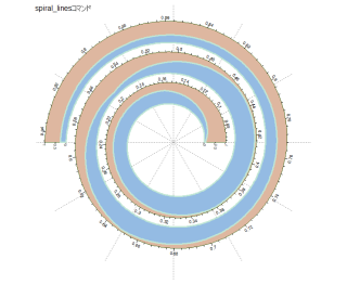
#折れ線グラフの描写:spiral_linesコマンド
#エリアを塗りつぶし:areaオプション;TRUE,FALSE
BasePlot()
spiral_lines(x = seq(max, min, length = 10), y = ValueRunif,
area = TRUE, type = "l",
gp = gpar(lwd = 3, fill = "#94bbe3",
col = "#bfe6d5", alpha = 1))
#スパイラルチャートタイトル
grid.text("spiral_linesコマンド", x = 0, y = 1, just = c("left", "top"))
#参考:軸に水平でプロット
#spiral_lines(x = seq(max, min, length = 10), y = runif(10),
# type = "h", gp = gpar(lwd = 3, col = "red"))
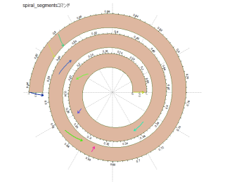
#セグメントを描写:spiral_segmentsコマンド
#矢印にする:arrowオプション
BasePlot()
spiral_segments(x0 = ValueRunif,
y0 = ValueRunif,
x1 = ValueRunif + runif(10, min = -0.02, max = 0.02),
y1 = 0.9 - ValueRunif, arrow = arrow(length = unit(2, "mm")),
gp = gpar(col = circlize::rand_color(10, luminosity = "bright"),
lwd = 2))
#スパイラルチャートタイトル
grid.text("spiral_segmentsコマンド", x = 0, y = 1, just = c("left", "top"))
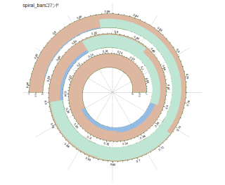
#棒グラフの描写:spiral_barsコマンド
#棒グラフの開始基準を指定:baselineオプション
BasePlot()
spiral_bars(pos = seq(0.3, 0.9, length = 10),
value = ValueRunif, baseline = 0,
gp = gpar(fill = ifelse(ValueRunif > 0.5, "#bfe6d5", "#94bbe3"), col = NA))
#スパイラルチャートタイトル
grid.text("spiral_barsコマンド", x = 0, y = 1, just = c("left", "top"))
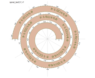
#テキストの描写:spiral_textコマンド
#描写方法の指定:facingオプション;"downward","inside","outside",
#"clockwise","reverse_clockwise","curved_inside","curved_outside"
BasePlot()
spiral_text(x = seq(0.3, 0.9, length = 10), y = 0.5,
"からだにいいもの", facing = "curved_inside",
gp = gpar(col = "#426617", alpha = 1))
#スパイラルチャートタイトル
grid.text("spiral_textコマンド", x = 0, y = 1, just = c("left", "top"))
#軸ラベルの追加:spiral_axisコマンド
BasePlot()
spiral_axis(major_at = seq(0, 1, length = 13),
labels = c("", month.name), minor_ticks = 6,
labels_gp = gpar(fontsize = 10, col = "red"))
#スパイラルチャートタイトル
grid.text("spiral_axisコマンド", x = 0, y = 1, just = c("left", "top"))
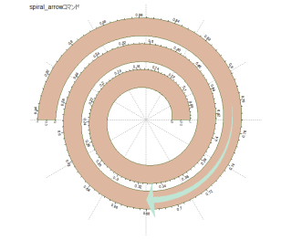
#矢印の描写:spiral_arrowコマンド
#矢印末端の形状:tailオプション;"normal","point"
#矢印の開始方向:arrow_position;"end","start"
#矢印先頭の幅:arrow_head_widthオプション
#矢印先頭の長さ:arrow_head_lengthオプション
BasePlot()
spiral_arrow(0.68, 0.78, tail = "point", arrow_position = "start",
arrow_head_width = 2, arrow_head_length = unit(4, "mm"),
gp = gpar(fill = "#bfe6d5", col = NA))
#スパイラルチャートタイトル
grid.text("spiral_arrowコマンド", x = 0, y = 1, just = c("left", "top"))
#画像を描写:spiral_rasterコマンド
#プロット方法の指定:facingオプション;"downward","inside","outside",
#"curved_inside","curved_outside"
#画像の読み込み
image <- system.file("extdata", "Rlogo.png", package = "circlize")
BasePlot()
spiral_raster(x = 0.3, y = 0.4, image, width = 0.05, height = 1,
facing = "curved_inside", nice_facing = TRUE)
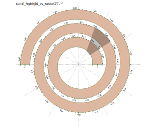
#指定エリアを塗りつぶし:spiral_highlight_by_sectorコマンド
BasePlot()
spiral_highlight_by_sector(x1 = 0.1, x2 = 0.12, x3 = 0.45, x4 = 0.48,
gp = gpar(fill = "black"))
#スパイラルチャートタイトル
grid.text("spiral_highlight_by_sectorコマンド",
x = 0, y = 1, just = c("left", "top"))
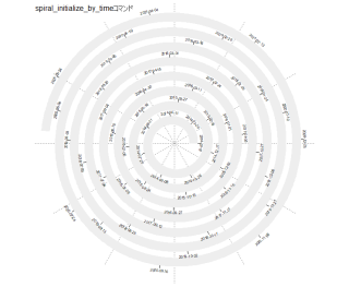
#日付軸のスパイラルチャートを作成:spiral_initialize_by_timeコマンド
#spiral_trackとspiral_axisコマンドと組み合わせて使用します。
#詳細はヘルプを確認してください
spiral_initialize_by_time(xlim = c("2014-01-01", "2021-06-17"))
spiral_track(height = 0.6)
spiral_axis()
#スパイラルチャートタイトル
grid.text("spiral_initialize_by_timeコマンド",
x = 0, y = 1, just = c("left", "top"))出力例
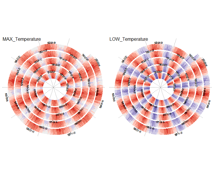
札幌の気温データを使用した例
気象庁HP:https://www.data.jma.go.jp/gmd/risk/obsdl/より札幌の気温データを取得・加工してプロットした例です。パソコンの性能によってはプロットに時間がかかります。
なお、ComplexHeatmapパッケージはBioconductorからインストールします。
使用したcsvデータは以下よりダウンロードできます。
#パッケージの読み込み
library("tcltk")
library("spiralize")
if(!require("tidyverse", quietly = TRUE)){
install.packages("tidyverse");require("tidyverse")}
if(!require("lubridate", quietly = TRUE)){
install.packages("lubridate");require("lubridate")}
if(!require("cowplot", quietly = TRUE)){
install.packages("cowplot");require("cowplot")}
if(!require("BiocManager", quietly = TRUE)){
install.packages("BiocManager");require("BiocManager")}
if(!require("ComplexHeatmap", quietly = TRUE)){
BiocManager::install("ComplexHeatmap");require("ComplexHeatmap")}
###データの準備#####
#気象庁HP:https://www.data.jma.go.jp/gmd/risk/obsdl/より札幌の気温データを取得・加工
#気温データは26298*3のサイズ
#SapporoTemp.csvを選択
FilePath <- paste0(as.character(tkgetOpenFile(title = "ファイルを選択",
filetypes = '{"ファイル" {".csv"}}',
initialfile = c("*.*"))), collapse = " ")
#読み込み
ReadData <- read.csv(FilePath)
#欠損値を0に置き換え,年月日で抽出
AnaData <- ReadData %>%
mutate_if(is.numeric, ~replace(., is.na(.), 0)) %>%
mutate(Date = ymd(Date)) %>%
filter(Date >= "1950-01-01" & Date <= "2000-12-31")
########
#cowplotパッケージでプロットするために空listを作成
PlotList <- list()
#cowplotパッケージでspiralizeパッケージのエラーを表示しない
spiral_opt$help = FALSE
#最高気温のスパイラルチャートを格納
PlotList[[1]] = grid.grabExpr({
#スパイラルチャート基本部分
spiral_initialize_by_time(xlim = range(AnaData[, 1]),
unit_on_axis = "days",
period = "years",
period_per_loop = 10,
polar_lines_by = 360/10) #,
#vp_param = list(x = unit(0, "npc"), just = "left"))
#トラックの追加
spiral_track(height = 0.8)
#気温のスパイラルチャート
lt = spiral_horizon(AnaData[, 1], AnaData[, 2], use_bar = TRUE,
pos_fill = "#D73027", neg_fill = "#313695")
#凡例の設定
#lgd = horizon_legend(lt, title = "MAX_Temperature")
#凡例の描写
#ComplexHeatmap::draw(lgd, x = unit(1, "npc") + unit(2, "mm"), just = "left")
#x軸の追加
spiral_axis(h = "top", curved_labels = TRUE, labels_gp = gpar(fontsize = 7))
#スパイラルチャートタイトル
grid.text("MAX_Temperature", x = 0, y = 1, just = c("left", "top"))
})
#最低気温のスパイラルチャートを格納
PlotList[[2]] = grid.grabExpr({
#スパイラルチャート基本部分
spiral_initialize_by_time(xlim = range(AnaData[, 1]),
unit_on_axis = "days",
period = "years",
period_per_loop = 10,
polar_lines_by = 360/10) #,
#vp_param = list(x = unit(0, "npc"), just = "left"))
#トラックの追加
spiral_track(height = 0.8)
#気温のスパイラルチャート
lt = spiral_horizon(AnaData[, 1], AnaData[, 3], use_bar = TRUE,
pos_fill = "#D73027", neg_fill = "#313695")
#凡例の設定
#lgd = horizon_legend(lt, title = "LOW_Temperature")
#凡例の描写
#ComplexHeatmap::draw(lgd, x = unit(1, "npc") + unit(2, "mm"), just = "left")
#x軸の追加
spiral_axis(h = "top", curved_labels = TRUE, labels_gp = gpar(fontsize = 7))
#スパイラルチャートタイトル
grid.text("LOW_Temperature", x = 0, y = 1, just = c("left", "top"))
})
#cowplotパッケージでプロット
plot_grid(plotlist = PlotList, ncol = 2, nrow = 1)出力例
少しでも、あなたの解析が楽になりますように!!