生存分析や競合リスク分析は、医学や生命科学などの分野で重要な課題です。これらの解析は患者の生存期間や複数のリスクを考慮した予測を行うため、診断や治療法の効果評価に不可欠です。しかし、これらの分析はデータが複雑で、専門的な知識が必要な上に、結果の可視化も難しくなります。
cifmodelingパッケージは、非パラメトリック推定や直接的な多項回帰(polytomous regression)を行うことで、生存確率や累積発生率関数(CIF)の推定が可能です。
また、”cifcurve”、”cifplot”、”cifpanel”などのコマンドで、リスクテーブルや競合リスクマークを含む高品質で複雑なレイアウトのプロットが可能です。
パッケージバージョンは0.9.8。Windows 11 x64 (build 26200)のR version 4.6.1で確認しています。

パッケージのインストール
下記コマンドを実行してください。
# パッケージのインストール
install.packages("cifmodeling")
# パッケージの読み込み
library("cifmodeling")
コマンド例
詳細はコメント、パッケージのヘルプを確認してください。
特定のイベントの生存時間データを抽出:extract_time_to_eventコマンド
| オプション | 意味 | 初期値 |
|---|---|---|
| formula | 生存時間とイベントの情報を指定するモデル式(Event(time, status)またはSurv(time, status)の左辺と、必要に応じてstrata()を含む)。 | なし(必須) |
| data | formulaで指定した変数を含むデータフレーム。 | なし(必須) |
| subset.condition | dataを絞り込む条件を文字列で指定(省略可能)。 | NULL |
| na.action | 欠測値の扱いを指定する関数。 | na.omit |
| which.event | 抽出するイベントの種類。”event1″(主要イベント)、”event2″(競合イベント)、”censor”/”censoring”(打ち切り)、”user_specified”(ユーザー指定)のいずれか。 | “event2” |
| code.event1, code.event2, code.censoring | 主要イベント・競合イベント・打ち切りに対応する整数コード。 | それぞれ1、2、0 |
| code.user.specified | which.event=”user_specified”の場合に抽出するイベントコード(例:中間イベントに3を指定)。 | NULL |
| read.unique.time | TRUEの場合、各層についてユニークかつソート済みの時間点のみを返す。 | TRUE |
| drop.empty | TRUEの場合、イベントが発生していない層は結果のリストから除外される。 | TRUE |
cifplotコマンドのオプション(一部抜粋):
| オプション | 意味 | 初期値 |
|---|---|---|
| formula_or_fit | モデル式(Event(time,status) ~ 層別化変数)、またはfit済みのsurvfitオブジェクト。 | なし(必須) |
| data | formulaで指定した変数を含むデータフレーム。 | NULL |
| outcome.type | アウトカムの種類。”survival”(カプラン・マイヤー)または”competing-risk”(アーレン・ヨハンセン)。省略時はイベント変数の水準数から自動判定される。 | 自動判定 |
| code.event1 | 主要イベントに対応する整数コード。 | 1 |
| code.event2 | 競合イベントに対応する整数コード。 | 2 |
| code.censoring | 打ち切りに対応する整数コード。 | 0 |
| label.x | x軸のラベル。 | “Time” |
| label.y | y軸のラベル。 | NULL(outcome.typeから自動決定) |
| add.conf | TRUEの場合、信頼区間のリボンを追加する。 | TRUE |
| add.risktable | TRUEの場合、プロット下にリスクテーブルを追加する。 | TRUE |
| add.censor.mark | TRUEの場合、各曲線に打ち切りマークを描画する。 | TRUE |
| add.competing.risk.mark | TRUEの場合、競合イベント(イベント2)が発生した時点にマークを描画する。 | FALSE |
| competing.risk.time | 競合イベントの発生時点を層ごとに格納した名前付きリスト。extract_time_to_event()の出力を渡すことが多い。 | list() |
| limits.y | y軸の範囲を指定する数値ベクトル(長さ2)。 | NULL(確率スケールではc(0,1)) |
# diabetes.complicationsデータセットを読み込む
data(diabetes.complications)

# 時間依存的生存分析の結果を抽出する関数を呼び出す
output <- extract_time_to_event(Event(t,epsilon) ~ fruitq,
                                data = diabetes.complications,
                                which.event = "event2")

# 競合リスクの累積発生率曲線をプロットする
cifplot(Event(t,epsilon) ~ fruitq,
        data = diabetes.complications,
        outcome.type="competing-risk",
        add.conf=FALSE,
        add.risktable=FALSE,
        add.censor.mark=FALSE,
        add.competing.risk.mark=TRUE,
        competing.risk.time=output,
        label.y="CIF of diabetic retinopathy",
        label.x="Years from registration")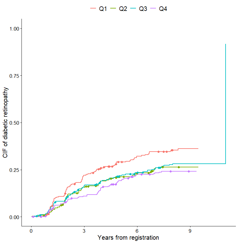
糖尿病患者のコホート研究データ
2型糖尿病患者に関する調査データです。糖尿病の併発症やその他の健康状態の分析に利用できます。
# diabetes.complicationsデータセットを読み込む
data(diabetes.complications)

# データセットの構造を表示する
str(diabetes.complications)
実行結果:
'data.frame':	978 obs. of  20 variables:
 $ t                : num  8.62 8.51 7.79 8.91 8.94 ...
 $ epsilon          : int  0 0 0 0 0 1 0 1 0 1 ...
 $ strata           : int  1 4 3 1 2 3 1 3 3 1 ...
 $ fruit            : num  75 26.8 64.3 5.35 211.05 ...
 $ fruitq1          : int  0 1 0 1 0 1 0 0 0 0 ...
 $ age              : int  45 68 63 49 55 61 56 64 67 58 ...
 $ sex              : int  0 0 0 0 0 0 0 1 1 1 ...
 $ bmi              : num  21.5 18.3 23.9 22.9 18.7 23.4 20.1 28.6 25.6 22.8 ...
 $ hba1c            : num  6.97 8.02 6.89 7.24 8.28 ...
 $ diabetes_duration: num  4.2 2.9 14.3 4.2 16.3 8.9 13 6.1 20.3 13.3 ...
 $ drug_oha         : int  0 0 1 1 1 1 0 1 0 0 ...
 $ drug_insulin     : int  0 1 0 0 0 0 1 0 0 1 ...
 $ sbp              : int  124 128 164 126 136 146 118 136 136 142 ...
 $ ldl              : num  187.3 87.6 74.6 95.7 50.5 ...
 $ hdl              : num  58.1 57.2 35 34.7 55.7 36.7 57.7 52.2 60.5 55.4 ...
 $ tg               : num  123 71 252 83 139 181 71 57 91 115 ...
 $ current_smoker   : int  0 1 1 1 1 0 1 0 0 0 ...
 $ alcohol_drinker  : int  0 0 1 0 0 0 0 0 0 0 ...
 $ ltpa             : num  52.5 11.03 4.38 9.38 12.38 ...
 $ fruitq           : Factor w/ 4 levels "Q1","Q2","Q3",..: 2 1 2 1 4 1 4 2 2 2 ...
前立腺がん試験データ
ステージ3〜4の前立腺がん患者を対象に、プラセボまたは異なる用量のエストロゲン投与(rx)による治療効果を比較した無作為化比較試験のデータです。治療法別の生存期間比較や、前立腺がんによる死亡とその他の原因による死亡を区別する競合リスク分析の例として利用できます。
# prostateデータセットを読み込む
data(prostate)

# 最初の観察値を表示する
head(prostate)
実行結果:
patno stage              rx dtime                 status age  wt
1     1     3 0.2 mg estrogen    72                  alive  75  76
2     2     3 0.2 mg estrogen     1        dead - other ca  54 116
3     3     3 5.0 mg estrogen    40 dead - cerebrovascular  69 102
4     4     3 0.2 mg estrogen    20 dead - cerebrovascular  75  94
5     5     3         placebo    65                  alive  67  99
6     6     3 0.2 mg estrogen    24    dead - prostatic ca  71  98
                    pf hx sbp dbp                           ekg       hg sz sg
1      normal activity  0  15   9                  heart strain 13.79883  2  8
2      normal activity  0  13   7 heart block or conduction def 14.59961 42 NA
3      normal activity  1  14   8                  heart strain 13.39844  3  9
4 in bed < 50% daytime  1  14   7                        benign 17.59766  4  8
5      normal activity  0  17  10                        normal 13.39844 34  8
6      normal activity  0  19  10                        normal 15.09961 10 11
         ap bm      sdate
1 0.2999878  0 1977-08-10
2 0.6999512  0 1977-09-21
3 0.2999878  0 1978-01-12
4 0.8999023  0 1978-03-19
5 0.5000000  0 1978-03-22

累積発生率(CIF)をプロット:cifcurveコマンド
| オプション | 意味 | 初期値 |
|---|---|---|
| formula | 生存時間とイベントの情報を指定するモデル式(Event(time,status)またはSurv(time,status)の左辺と、層別化変数の右辺)。cifplot()と異なり、fit済みのsurvfitオブジェクトは受け付けない。 | なし(必須) |
| data | formulaで指定した変数を含むデータフレーム。 | なし(必須) |
| weights | dataに含まれる重み変数の名前(省略可能、非負値)。 | NULL |
| n.risk.type | リスク集合のサイズ$n.riskの算出方法。”weighted”、”unweighted”、”ess”のいずれか(推定値・標準誤差には影響しない)。 | “weighted” |
| subset.condition | dataを絞り込む条件を文字列で指定(省略可能)。 | NULL |
| na.action | 欠測値の扱いを指定する関数。 | na.omit |
| outcome.type | アウトカムの種類。”survival”(カプラン・マイヤー)または”competing-risk”(アーレン・ヨハンセン)。NULLの場合、イベント変数の水準数から自動判定される。 | NULL(自動判定) |
| time.point | null.hypothesis指定時に片側検定を行う時点(省略可能)。 | NULL |
| null.hypothesis | time.pointにおける生存確率またはCIFの帰無仮説値(省略可能)。 | NULL |
| code.event1 | 主要イベントに対応する整数コード。 | 1 |
| code.event2 | 競合イベントに対応する整数コード。 | 2 |
| code.censoring | 打ち切りに対応する整数コード。 | 0 |
| error | 標準誤差・信頼区間の算出方法。生存の場合は”greenwood”/”tsiatis”/”if”、競合リスクの場合は”delta”/”aalen”/”if”から選択(重み付き解析では”if”が推奨)。 | NULL(生存: “greenwood”、競合リスク: “delta”) |
| conf.type | 信頼区間の変換方法。 | “arcsine-square root” |
| conf.int | 信頼区間の両側水準。 | 0.95 |
| report.influence.function | TRUEの場合、影響関数も計算して返す(engine=”calculateAJ_Rcpp”の場合のみ)。 | FALSE |
| report.survfit.std.err | TRUEの場合、標準誤差をsurvfitの慣例に合わせ対数生存スケールで報告する。 | FALSE |
| engine | 内部計算エンジン。”auto”、”calculateKM”、”calculateAJ_Rcpp”のいずれか。 | “calculateAJ_Rcpp” |
| prob.bound | 確率を0・1から離すために内部的に用いる下限値。 | 1e-07 |
# diabetes.complicationsデータセットを読み込む
data(diabetes.complications)

# 競合リスクの累積発生率曲線を計算する
output1 <- cifcurve(Event(t,epsilon) ~ fruitq,
                    data = diabetes.complications,
                    outcome.type="competing-risk")

# 競合リスクの累積発生率曲線をプロットする
cifplot(output1,
        outcome.type = "competing-risk",
        type.y = "risk",
        add.risktable = FALSE,
        label.y = "CIF of diabetic retinopathy",
        label.x = "Years from registration")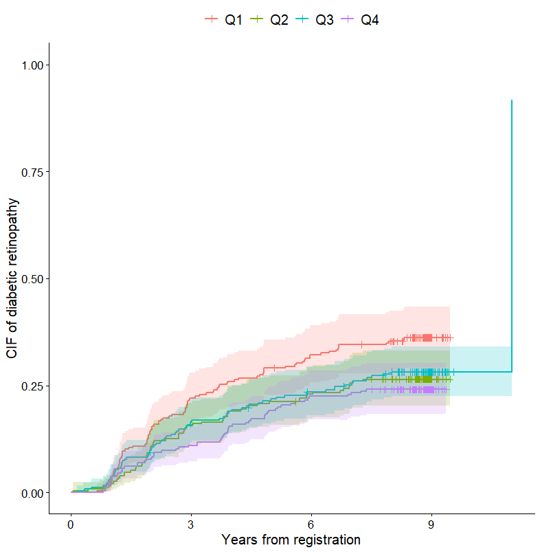
生存や競合リスクの応答をプロット:polyregコマンド
| オプション | 意味 | 初期値 |
|---|---|---|
| nuisance.model | アウトカムと(曝露変数を除く)調整共変量を指定するモデル式。左辺はEvent(time,status)またはSurv(time,status)。 | なし(必須) |
| exposure | dataに含まれるカテゴリカルな曝露変数の名前。 | なし(必須) |
| strata | 従属的な打ち切りを調整するための層別化変数の名前(省略可能)。 | NULL |
| data | アウトカム・曝露・調整共変量を含むデータフレーム。 | なし(必須) |
| code.event1 | 主要イベントに対応する整数コード。 | 1 |
| code.event2 | 競合イベントに対応する整数コード。 | 2 |
| code.censoring | 打ち切りに対応する整数コード。 | 0 |
| code.exposure.ref | 曝露の基準カテゴリに対応する整数コード。 | 0 |
| effect.measure1 | 主要イベントの効果指標。”RR”(リスク比)、”OR”(オッズ比)、”SHR”(部分分布ハザード比)から選択。 | “RR” |
| effect.measure2 | 競合イベントの効果指標。”RR”、”OR”、”SHR”から選択。 | “RR” |
| time.point | 曝露効果を評価する時点。outcome.typeが”competing-risk”または”survival”の場合は必須。 | NULL |
| outcome.type | アウトカムの種類。”competing-risk”、”survival”、”binomial”、”proportional-survival”、”proportional-competing-risk”のいずれか。 | “competing-risk” |
| conf.int | 信頼区間の両側水準。 | 0.95 |
# イベントコード:0=打ち切り、1=主要イベント、2=競合イベント
# diabetes.complicationsデータセットを読み込む
data(diabetes.complications)

# 多項回帰分析を実行する
output <- polyreg(
  nuisance.model = Event(t, epsilon) ~ +1,
  exposure = "fruitq1",
  data = diabetes.complications,
  effect.measure1 = "RR",
  effect.measure2 = "RR",
  time.point = 8,
  outcome.type = "competing-risk"
)

# 結果:長いので省略
output
多項ロジットモデルを使用した累積発生率の回帰分析例
# diabetes.complicationsデータセットを読み込む
data(diabetes.complications)

# 多項回帰分析を実行する
output <- polyreg(
  nuisance.model = Event(t, epsilon) ~ +1,
  exposure = "fruitq1",
  data = diabetes.complications,
  effect.measure1 = "RR",
  effect.measure2 = "RR",
  time.point = 8,
  outcome.type = "competing-risk"
)

# 回帰モデルの係数を表示する
coef(output)
# 回帰モデルの共分散行列を表示する
vcov(output)
# 使用された観察値の数を表示する
nobs(output)
# 回帰モデルの要約結果を表示する
summary(output)
実行結果:
[1] -1.38313159  0.30043942 -3.99147406  0.07582595
             [,1]         [,2]         [,3]         [,4]
[1,]  0.007132823 -0.004524224  0.002772872 -0.002210804
[2,] -0.004524224  0.009639840 -0.001178880  0.004588230
[3,]  0.002772872 -0.001178880  0.018638168 -0.016918563
[4,] -0.002210804  0.004588230 -0.016918563  0.054838178
[1] 978

                      event1        event2
----------------------------------------------
fruitq1, 1 vs 0
                      1.350         1.079
                      [1.114, 1.637]  [0.682, 1.707]
                      (p=0.002)     (p=0.746)

----------------------------------------------

effect.measure        RR at 8       RR at 8
n.events              279 in N = 978  79 in N = 978
median.follow.up      8             -
…(以下略)
複数の生存と累積発生率プロットをパネル表示にする例
この関数は、複数の生存曲線とCIFプロットをパネル表示に配置します。結果として得られるグラフは、複数の生存パターンを一度に比較できます。
| オプション | 意味 | 初期値 |
|---|---|---|
| plots | パネルにまとめる既存のggplotオブジェクトのリスト。指定した場合、新たにモデルは当てはめず、そのまま配置される。 | NULL |
| formula | モデル式(Event(time,status) ~ 層別化変数)。cifplot()と異なり、fit済みのsurvfitオブジェクトは受け付けない。 | NULL |
| data | formulaで指定した変数を含むデータフレーム。 | NULL |
| outcome.type | アウトカムの種類。”survival”または”competing-risk”。 | NULL(自動判定) |
| code.events | イベント・打ち切りコードの指定。競合リスクではc(event1, event2, censoring)、複数パネルの場合はそのベクトルのリストを指定できる。 | NULL |
| label.y | y軸のラベル(パネルごとに指定可能)。 | NULL |
| label.x | x軸のラベル(パネルごとに指定可能)。 | NULL |
| rows.columns.panel | パネルの行数・列数を指定する整数ベクトルc(nrow, ncol)。 | c(1, 1) |
| inset.panel | TRUEの場合、1つ目のプロットをメインに、2つ目のプロットをインセット(挿入図)として重ねて表示する(3つ目以降は無視される)。 | FALSE |
| title.panel | パネル全体に付けるタイトル。 | NULL |
| subtitle.panel | パネル全体に付けるサブタイトル。 | NULL |
| caption.panel | パネル全体に付けるキャプション。 | NULL |
| title.plot | 各パネルに付けるタイトルのベクトル(描画順に対応。インセットモードでは1つ目がメイン、2つ目がインセット)。 | NULL |
| legend.position | 凡例の位置。”top”、”right”、”bottom”、”left”、”none”のいずれか。 | “top” |
| legend.collect | TRUEの場合、全パネルで凡例を1つにまとめる。 | TRUE |
| inset.left, inset.right | インセットの水平位置を基準領域に対する割合(0〜1)で指定。 | 0.6、0.98 |
| inset.bottom, inset.top | インセットの垂直位置を基準領域に対する割合(0〜1)で指定。 | 0.05、0.45 |
| inset.align.to | インセットの基準とする座標系。”panel”(プロット領域)、”plot”(軸・タイトルを含む全体)、”full”(キャンバス全体)のいずれか。 | “panel” |
| inset.legend.position | インセットのプロットのみに適用する凡例位置。NULLの場合、インセット側で設定された凡例位置がそのまま使われる。 | NULL |
# diabetes.complicationsデータセットを読み込む
data(diabetes.complications)

# 競合リスクの累積発生率曲線をパネル形式でプロットするためのオブジェクトを作成する
output1 <- cifpanel(
  title.panel = "A comparison of cumulative incidence of competing events",
  rows.columns.panel = c(1,2),
  formula = Event(t, epsilon) ~ fruitq,
  data = diabetes.complications,
  outcome.type = "competing-risk",
  code.events = list(c(1,2,0), c(2,1,0)),
  label.y = c("Diabetic retinopathy", "Macrovascular complications"),
  label.x = "Years from registration",
  subtitle.panel = "Stratified by fruit intake",
  caption.panel  = "Data: diabetes.complications",
  title.plot = c("Diabetic retinopathy", "Macrovascular complications"),
  legend.position = "bottom",
  legend.collect=TRUE
)

# パネル形式のプロットを表示する
print(output1)

# 競合リスクの累積発生率曲線を個別にプロットする(1つ目:糖尿病網膜症)
output2 <- cifplot(Event(t,epsilon) ~ fruitq,
                   data = diabetes.complications,
                   outcome.type="competing-risk",
                   code.event1=2,
                   code.event2=1,
                   add.conf = FALSE,
                   add.risktable = FALSE,
                   label.y="CIF of macrovascular complications",
                   label.x="Years from registration")

# 競合リスクの累積発生率曲線を個別にプロットする(2つ目:インセット表示用にy軸を制限)
output3 <- cifplot(Event(t,epsilon) ~ fruitq,
                   data = diabetes.complications,
                   outcome.type="competing-risk",
                   code.event1=2,
                   code.event2=1,
                   add.conf = FALSE,
                   add.risktable = FALSE,
                   label.y="",
                   label.x="",
                   limits.y=c(0,0.15))
# 警告メッセージが出ても問題なし
# 警告メッセージ:
# Some point estimates fall outside `limits.y` = [0, 0.15].

# 2つのプロットをリストにまとめる
output4 <- list(a = output2$plot, b = output3$plot)

# 個別のプロットをパネル形式で表示する
output5 <- cifpanel(plots = output4,
                    inset.panel = TRUE,
                    inset.left = 0.40, inset.bottom = 0.45,
                    inset.right = 1.00, inset.top = 0.95,
                    inset.align.to = "plot",
                    inset.legend.position = "none",
                    legend.position = "bottom")
# パネル形式のプロットを表示する
print(output5)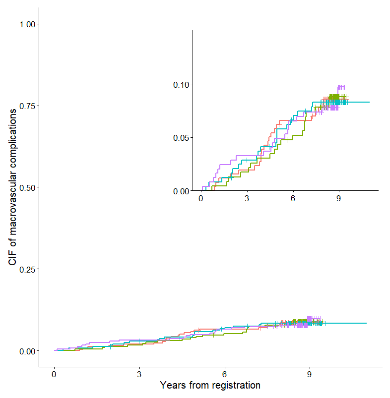
この記事が誰かの役に立ちますように。