本パッケージに収録されている多くのコマンドは「基本的なコマンドを組み合わせる」ことで再現が可能です。でも、再現しようとすると手がかかります。なお、「broman」パッケージ名の由来は作者が「Broman」氏だからです。
抄録されているコマンドから目に付いたものを紹介します。他のコマンドはパッケージヘルプを参照ください。
パッケージのバージョンは0.59-5。R version 3.2.1でコマンドを確認しています。
パッケージのインストール
下記コマンドを実行してください。
#パッケージのインストール
install.packages("broman")
実行コマンドの紹介
詳細はコメント、パッケージヘルプを確認してください。
#パッケージの読み込み
library("broman")
#数字にカンマを加える:add_commasコマンド
#注意出力が文字列になります
add_commas(c(1, 22, 444, 5555, 66666, 666666))
[1] "1" "22" "444" "5,555" "66,666" "666,666"
#マウスで任意の場所に矢印を図に加える:arrowlocatorコマンド
#1回目のクリックで始点、2回目のクリックで終点を指定します
plot(0, 0, type = "n", xlab = "", ylab = "", xlim = c(0, 1), ylim = c(0, 1))
arrowlocator(col = "blue", lwd = 2)
#一致を調査:cfコマンド
#matrix, data.frame, list, vectorの調査が可能です
x <- c(5, 8, 9, NA, 3, NA)
y <- c(5, 2, 9, 4, NA, NA)
cf(x,y)
[1] TRUE FALSE TRUE FALSE FALSE TRUE
#指定した色,alpha値のカラーコードを取得:colwalphaコマンド
colwalpha(c("blue", "red"), alpha = 0.5)
[1] "#0000FF7F" "#FF00007F"
#行列の行方向配列の一致を調査:compare_rowsコマンド
#methodオプション:prop_mismatches;一致は1,不一致0,
# rms_difference;比較対象との差分
y <- matrix(sample(1:4, 5, replace=TRUE), ncol = 1)
[,1]
[1,] 3
[2,] 1
[3,] 4
[4,] 2
[5,] 3
compare_rows(y, method = "rms_difference")
[,1]
[1,] 3
[2,] 1
[3,] 4
[4,] 2
[5,] 3
#数値を16進数に変換:convert2
convert2hex(333)
[1] "14d"
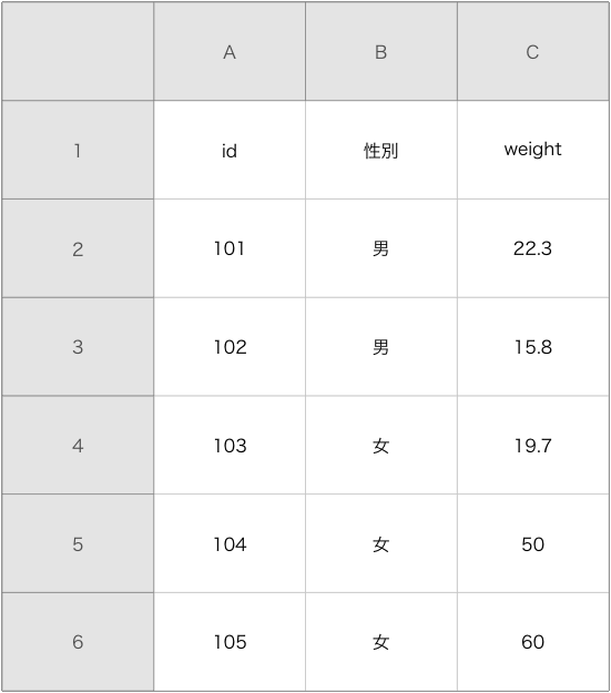
#データフレームの内容をエクセル風にプロット:excel_fig
df <- data.frame(id = c(101, 102, 103, 104, 105),
"性別" = c("男", "男", "女", "女", "女"),
weight = c(22.3, 15.8, 19.7, 50, 60),
stringsAsFactors = FALSE)
#Macで文字化け防止
par(family = "HiraKakuProN-W3")
#プロット
excel_fig(df, col_names = TRUE)
#Rの終了:exitコマンド
#注意:RStudioで使用すると強制終了します
exit()
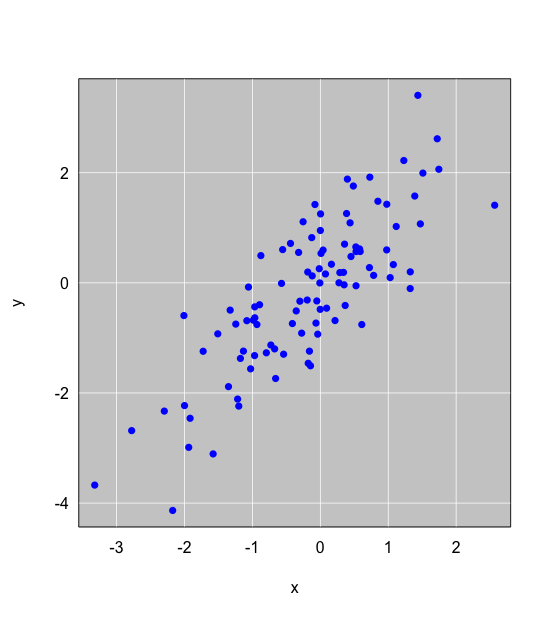
#plotコマンドでggplot2風の図をプロット:grayplotコマンド
x <- rnorm(100)
y <- x + rnorm(100, 0, 0.7)
grayplot(x, y, col = "blue", pch = 16)
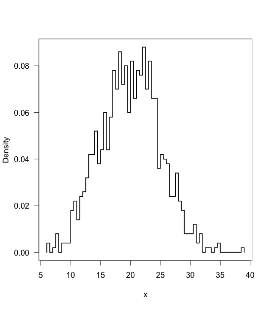
#histグラムを描写:histlinesコマンド
x <- rnorm(1000, mean = 20, sd = 5)
plot(histlines(x, breaks = 60, use = "density"),
type = "l", lwd = 2, xlab = "x", ylab = "Density", las = 1)
#今日の日付けを取得:kbdateコマンド
#formatオプション:dateonly;年月日,standard;曜日月時間年
kbdate("standard")
#windowsでの出力
[1] "木 8 06 22:51:39 2015"
#macでの出力
[1] "木 8 06 22時51分53秒 2015"
#重複するデータの数を表示:lenuniqコマンド
x <- c(1, 2, 1, 3, 1, 1, 2, 2, 3, NA, NA, 1)
lenuniq(x, na.rm = FALSE)
[1] 4
#小数点以下の桁数を指定:myroundコマンド
myround(51.01, digits = 10)
[1] "51.0100000000"
#変数を.で結合:paste.コマンド
x <- 3
y <- 4
paste.(x, y)
[1] "3.4"
#下記と同じ
paste(x, y, sep = ".")
[1] "3.4"
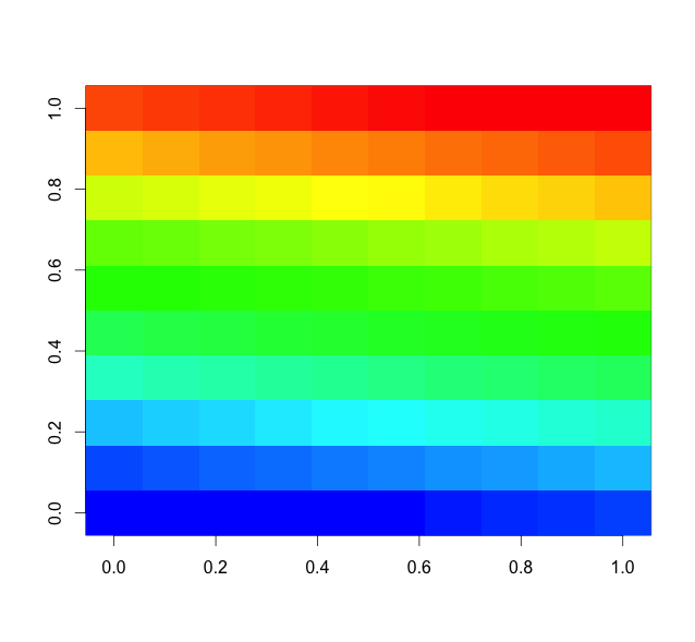
#赤から青のカラーパレットを作成:revrainbowコマンド
x <- matrix(1:100, ncol = 10)
image(x, col = revrainbow())出力例
・excel_figコマンド
・grayplotコマンド
・histlinesコマンド
・revrainbowコマンド
少しでも、あなたのウェブや実験の解析が楽になりますように!!