日本の行政地区をプロットするのに便利なパッケージの紹介です。
パッケージバージョンは0.3.0。windows 10のR version 3.4.3で動作を確認しています。
パッケージのインストール
下記コマンドを実行してください。
#パッケージのインストール
install.packages("jpndistrict")
コマンドの紹介
詳細はコマンド、パッケージのヘルプを確認してください。
#パッケージの読み込み
library("jpndistrict")
#install.packages("devtools")
#sfオブジェクトを利用するためにgithubからggplot2をインストール
#devtools::install_github("tidyverse/ggplot2")
library("ggplot2")
#shinyでインタラクティブに行政区間を確認:district_viewerコマンド
district_viewer()
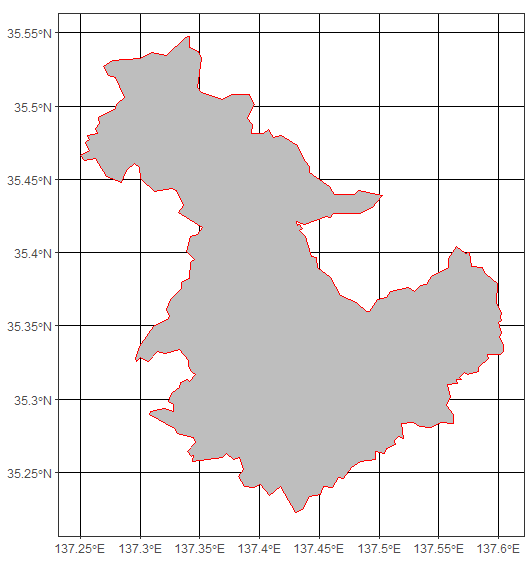
#経度緯度から行政区都道府県市名の情報を取得:find_cityコマンド
GetCity <- find_city(longitude = 137.5993, latitude = 35.36358)
#確認
GetCity
Simple feature collection with 1 feature and 3 fields
geometry type: POLYGON
dimension: XY
bbox: xmin: 137.2497 ymin: 35.22276 xmax: 137.604 ymax: 35.54718
epsg (SRID): 4326
proj4string: +proj=longlat +datum=WGS84 +no_defs
# A tibble: 1 x 4
prefecture city_code city geometry
<chr> <chr> <chr> <S3: sfc_POLYGON>
1 岐阜県 21210 恵那市 <S3: sfc_POLYGON>
#ggplot2パッケージ
ggplot(GetCity, aes(geometry = geometry)) +
geom_sf(col = "red", fill = "gray") +
theme_bw()
#plotコマンド
plot(GetCity$geometry, col = "gray")
########
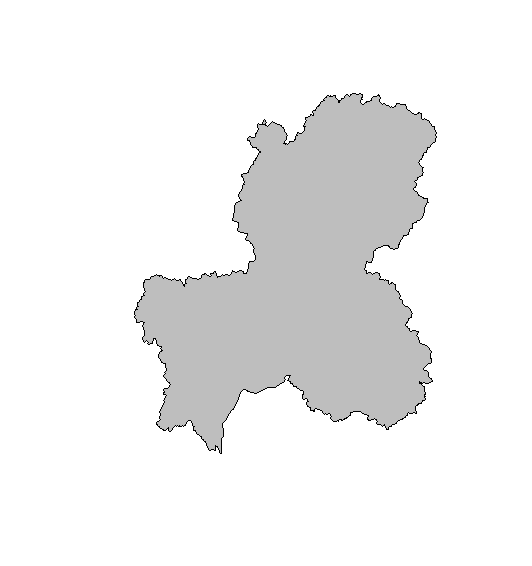
#経度緯度から行政区都道府県の情報を取得:find_prefコマンド
GetPref <- find_pref(longitude = 137.5993, latitude = 35.36358)
#結果
GetPref
Simple feature collection with 1 feature and 2 fields
geometry type: POLYGON
dimension: XY
bbox: xmin: 136.2751 ymin: 35.13267 xmax: 137.6542 ymax: 36.46616
epsg (SRID): 4326
proj4string: +proj=longlat +datum=WGS84 +no_defs
# A tibble: 1 x 3
pref_code prefecture geometry
<chr> <chr> <S3: sfc_POLYGON>
1 21 岐阜県 <S3: sfc_POLYGON>
#ggplot2パッケージ
ggplot(GetPref, aes(geometry = geometry)) +
geom_sf(col = "red", fill = "gray") +
theme_bw()
#plotコマンド
plot(GetPref$geometry, col = "gray")
########
#経度緯度に含まれる行政区都道府県の情報を取得:find_prefsコマンド
GetPrefs <- find_prefs(longitude = 137.5993, latitude = 35.36358)
#結果
GetPrefs
# A tibble: 3 x 4
pref_code meshcode_80km prefecture region
<chr> <dbl> <fctr> <chr>
1 20 5337 長野県 中部
2 21 5337 岐阜県 中部
3 23 5337 愛知県 中部
#######
#行政区都道府県のjis_code,経度緯度等のデータセット:jpnprefsコマンド
jpnprefs
# A tibble: 47 x 7
jis_code prefecture capital region major_island capital_latitude capital_longitude
<chr> <fctr> <chr> <chr> <chr> <dbl> <dbl>
1 01 北海道 札幌市 北海道 北海道 43.06208 141.3544
2 02 青森県 青森市 東北 本州 40.82200 140.7472
3 03 岩手県 盛岡市 東北 本州 39.70197 141.1544
4 04 宮城県 仙台市 東北 本州 38.26811 140.8693
5 05 秋田県 秋田市 東北 本州 39.71975 140.1022
6 06 山形県 山形市 東北 本州 38.25539 140.3395
7 07 福島県 福島市 東北 本州 37.76089 140.4734
8 08 茨城県 水戸市 関東 本州 36.36583 140.4711
9 09 栃木県 宇都宮市 関東 本州 36.55503 139.8828
10 10 群馬県 前橋市 関東 本州 36.38936 139.0633
# ... with 37 more rows
#######
#jis_codeで情報を取得:jpn_citiesコマンド
GetCities <- jpn_cities(jis_code = 21)
#行政区市町村名を確認
GetCities$city
[1] "岐阜市" "大垣市" "高山市" "多治見市" "関市" "中津川市" "美濃市"
[8] "瑞浪市" "羽島市" "恵那市" "美濃加茂市" "土岐市" "各務原市" "可児市"
[15] "山県市" "瑞穂市" "飛騨市" "本巣市" "郡上市" "下呂市" "海津市"
[22] "羽島郡 岐南町" "羽島郡 笠松町" "養老郡 養老町" "不破郡 垂井町" "不破郡 関ケ原町" "安八郡 神戸町" "安八郡 輪之内町"
[29] "安八郡 安八町" "揖斐郡 揖斐川町" "揖斐郡 大野町" "揖斐郡 池田町" "本巣郡 北方町" "加茂郡 坂祝町" "加茂郡 富加町"
[36] "加茂郡 川辺町" "加茂郡 七宗町" "加茂郡 八百津町" "加茂郡 白川町" "加茂郡 東白川村" "可児郡 御嵩町" "大野郡 白川村"
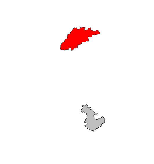
#参考例:市町村を指定してプロット
PlotData <- subset(GetCities, GetCities$city == "恵那市" | GetCities$city == "飛騨市")
plot(PlotData$geometry, col = c("gray", "red"))
#######出力例
・find_cityコマンド:ggplot2パッケージを利用
・find_prefコマンド
・jpn_citiesコマンド
少しでも、あなたの解析が楽になりますように!!