データ集計でよく使っている「tidyverse」パッケージのコマンドです。マニアックなことはしていません。数は少ないですが基本的な内容です。
パッケージバージョンは1.2.1。windows 10のR version 3.5.2で動作を確認しています。
パッケージのインストール
下記コマンドを実行してください。
install.packages("tidyverse")データ例の作成
Rに標準で用意されているirisを変更して使用します。下記コマンドを実行してください。
#tibble形式に変換
as.tibble(iris) %>%
 #id情報を付与
rowid_to_column(var = "ID") %>%
 #Speciesに"_色情報"を付与
mutate(Species = str_c(Species,
c("red", "yellow", "blue"),
sep = "_")) %>%
 #列名Speciesを"Species_Color"に変更
 rename("Species_Color" = Species) %>%
 #データ順を変更
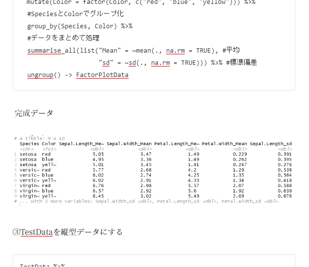
select(ID, Species_Color, everything()) -> TestData完成データ
データの操作例
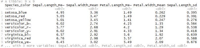
①Species_Colorごとの統計量を算出する。
TestData %>%
 #IDを除去
  select(-ID) %>%
 #Species_Colorでグループ化
  group_by(Species_Color) %>%
 #データをまとめて処理
  summarise_all(list("Mean" = ~mean(., na.rm = TRUE), #平均
                     "sd" = ~sd(., na.rm = TRUE))) %>% #標準偏差
  ungroup() -> PlotData
完成データ
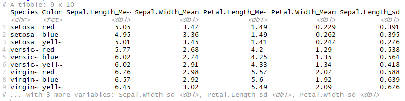
②Spcies_Colorデータを”Species”と”Color”に分割し
“Color” をred,yellow,blueの順序を持つFactorに変換後、 “Species”と”Color” ごとの統計量を算出する。
TestData %>%
  #IDを除去
  select(-ID) %>%
  #Species_Colorを"_"で分割
  separate(Species_Color, into = c("Species", "Color"), sep = "_") %>%
  #Colorをred,blue,yellowの順序を持つFactor化
 mutate(Color = factor(Color, c("red", "blue", "yellow"))) %>%
  #SpeciesとColorでグループ化
  group_by(Species, Color) %>%
  #データをまとめて処理
  summarise_all(list("Mean" = ~mean(., na.rm = TRUE), #平均
                     "sd" = ~sd(., na.rm = TRUE))) %>% #標準偏差
  ungroup() -> FactorPlotData
完成データ
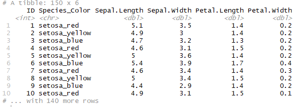
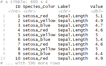
③TestDataを縦型データにする
TestData %>%
  gather(key = "Label", value = "Value",
     -ID, -Species_Color) -> GatherData
完成データ
④GatherDataを横型データにする
GatherData %>%
  spread(key = Label, value = Value)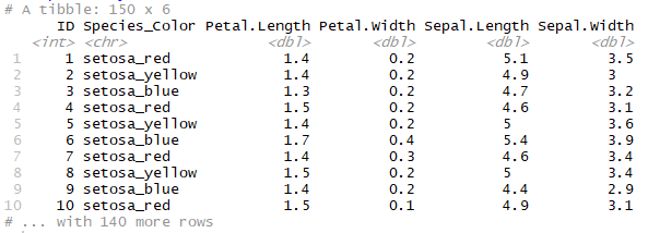
少しでも、あなたの解析が楽になりますように!!