区間データ分析は、価格帯やエンジン排気量など、単一の値ではなく最小値・最大値といった範囲で表されるデータを扱う分野です。これらのデータは具体的な値ではなく範囲として表されるため、通常の統計手法では適切に解析できないことがあります。AIDAパッケージは、このような区間データの構築、可視化、そして統計的モデリングを支援します。
このパッケージを使えば、’intData’クラスを使って区間データを表現し、マイクロデータを集約したり、潜在分布のパラメータを推定することが可能になります。また、Mallows距離に基づいた重心(バリセンター)や共分散行列の推定、そして区間最小共分散行列式(IMCD)によるロバストな共分散行列の推定も提供しています。
特に、外れ値検出やデータの可視化を得意としています。区間データを効率的に分析し、より正確な結果を得ることができます。
パッケージバージョンは0.2.0。Windows 11 x64 (build 26200)のR version 4.6.0で確認しています。

パッケージのインストール
下記コマンドを実行してください。
# パッケージのインストール
install.packages("AIDA")
# パッケージの読み込み
library("AIDA")
コマンド例
詳細はコメント、パッケージのヘルプを確認してください。
区間データのShapley分解を棒グラフで可視化:plot_bar_int_Shapley_decompコマンド
| オプション | 意味 | 初期値 |
|---|---|---|
| shapley_decomp | 観察値ごとのShapley値の寄与を含む行列のリスト。 | |
| palette | 各特徴量の色。paletteがNULLの場合、RColorBrewerを使用して生成される。 | NULL |
| rotate_x | 論理値。TRUEの場合、x軸ラベルが回転する。 | TRUE |
| abbrev.obs | 整数。abbrev.obs > 0の場合、行名はabbreviateでminlength = abbrev.obsで省略される。 | 20 |
| sort.obs | 論理値。TRUEの場合、観察値は総Shapley値に従ってソートされる。 | TRUE |
| plot_IMah | 論理値。TRUEの場合、区間マハラノビス距離(全Shapley値の和)がプロットに含まれる。 | FALSE |
# creditcardデータセットを読み込む
data(creditcard)
# intDataオブジェクトを作成
credit_card_int <- creditcard$intData
# Shapley分解を計算(IMCD推定に基づき、中心・範囲・交差項の寄与に分解)
credit_card_shap_decomp <- int_Shapley_decomp(credit_card_int)
# Shapley分解の棒グラフをプロット
plot_bar_int_Shapley_decomp(credit_card_shap_decomp,
                            palette = rainbow(credit_card_int@NIVar))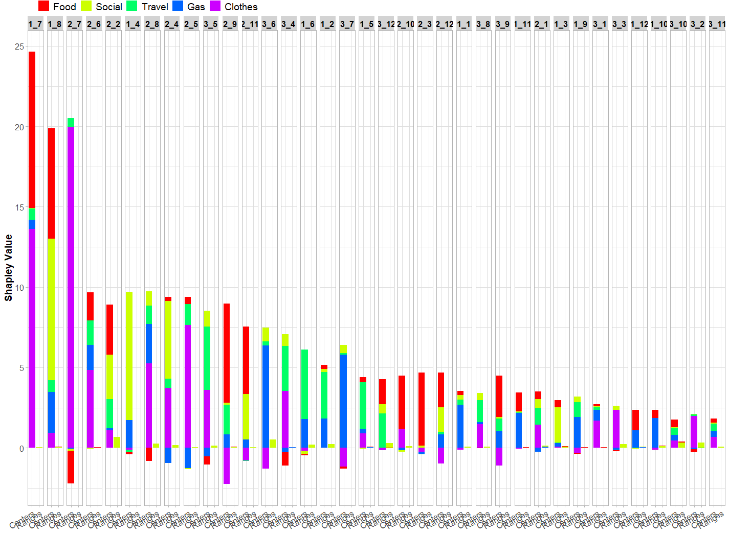
区間データのペアプロットを作成:plot_pairs_intコマンド
区間データのペアプロットを作成します。データ点を長方形や交差記号で表示し、相関係数を可視化できます。
| オプション | 意味 | 初期値 |
|---|---|---|
| data | マイクロデータ/区間データを含むintDataオブジェクト。 | |
| type | 生成するプロットのタイプ:”rectangles”、”crosses”、または”crosses2″。デフォルトは”rectangles”。 | c(“rectangles”, “crosses”, “crosses2”) |
| cex.cor | 文字拡大率 | 2 |
| corr | シンボリック相関を含む行列。提供されない場合、上部パネルが省略される。 | NULL |
| palette | 各観測値の色を指定。 | rainbow(nrow(data)) |
| fill_col | type=”rectangles”の場合、各観測値の塗りつぶし色または全観測値に適用する単一の色を指定。デフォルトは”gray50″。 | “gray50” |
| is_outlier | 外れ値かどうかを示す論理値ベクトル。外れ値の線幅を太くします。デフォルトはNULL。 | NULL |
# creditcardデータセットを読み込む
data(creditcard)
# intDataオブジェクトを作成
credit_card_int <- creditcard$intData
# 共分散行列を計算
credit_card_cov <- int_cov(credit_card_int)
# 相関行列を計算
credit_card_cor <- cov2cor(credit_card_cov)
# 散布図ペアプロットを表示
plot_pairs_int(credit_card_int,
               corr = credit_card_cor,
               labels = colnames(credit_card_int))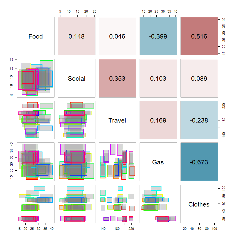
区間データの散布図を作成し、外れ値を強調する:plot_scatter_intコマンド
| オプション | 意味 | 初期値 |
|---|---|---|
| data | マイクロデータ/区間データを含むintDataオブジェクト。最初の2つの変数がx軸とy軸に使用されます。 | |
| type | 生成するプロットのタイプ:”rectangles”、”crosses”、または”crosses2″。デフォルトは”rectangles”。 | c(“rectangles”, “crosses”, “crosses2”) |
| palette | 各観測値の色を指定。デフォルトはrainbow(nrow(data))。 | rainbow(nrow(data)) |
| fill_col | type=”rectangles”の場合、各観測値の塗りつぶし色または全観測値に適用する単一の色を指定。デフォルトは”gray50″。 | “gray50” |
| is_outlier | 外れ値かどうかを示す論理値ベクトル。外れ値の線幅を太くします。デフォルトはNULL。 | NULL |
# creditcardデータセットを読み込む
data(creditcard)
# intDataオブジェクトを作成
credit_card_int <- creditcard$intData
# いったん散布図を表示
plot_scatter_int(credit_card_int[, c(3, 5)])

# 外れ値を強調するデータを計算
# ロバストな距離を計算(IMCD推定に基づく)
credit_card_dist <- IMah_dist(credit_card_int)
# 外れ値を検出
credit_card_outliers <- int_outliers(credit_card_dist, "farness", 0.9)

# 外れ値の色を設定
outliers_colors <- rep('gray50', credit_card_int@NObs)
names(outliers_colors) <- rownames(credit_card_int)
outliers_colors[credit_card_outliers$outliers_names] = 'red'

# 外れ値を強調した散布図を上書き
plot_scatter_int(credit_card_int[, c(3, 5)],
                 palette = outliers_colors,
                 is_outlier = credit_card_outliers$is_outlier)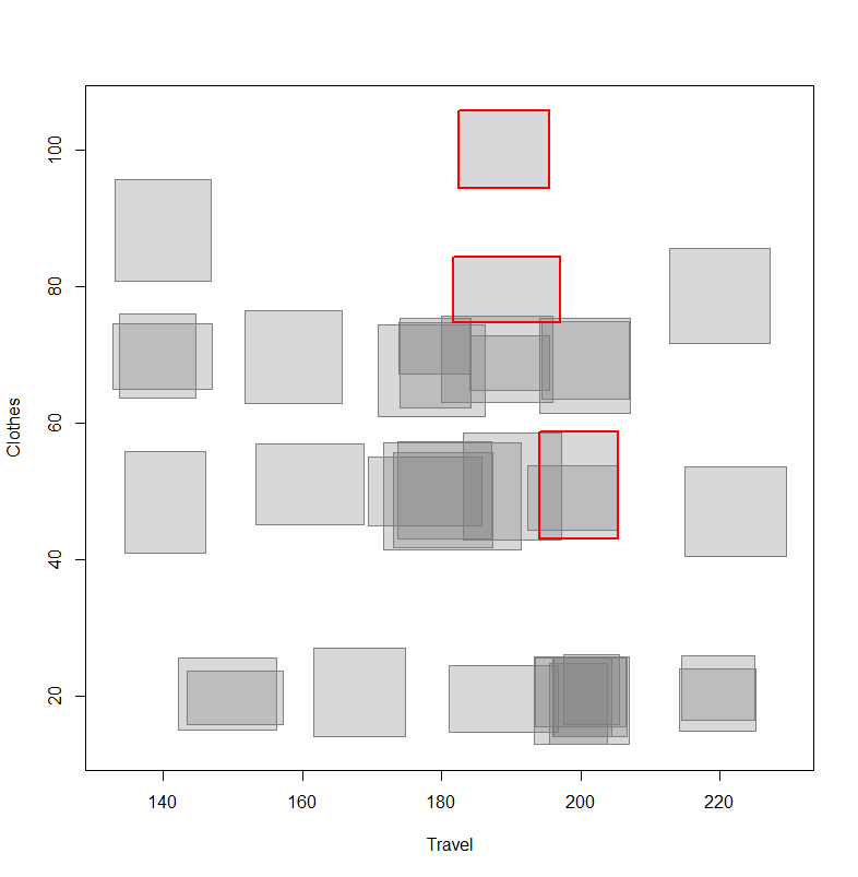
<おすすめのRに関する書籍です>

Rではじめるデータサイエンス 第2版 | Hadley Wickham, Mine Çetinkaya-Rundel, Garrett Grolemund, 大橋 真也
Rによる機械学習[第3版] (Programmer's SELECTION)
区間データのShapley値の棒グラフをプロット:plot_bar_int_Shapleyコマンド
| オプション | 意味 | 初期値 |
|---|---|---|
| x | n個の観測値とp個の変数に対するShapley値を含むn x p行列。 | |
| cutoff_value | 外れ値検出に使用するカットオフ値。cutoff_valueがNULLでない場合(デフォルト)、カットオフ値はプロットに含まれます。 | NULL |
| cutoff_label | カットオフ値線のラベルを指定。 | NULL |
| palette | 各変数の色を指定。paletteがNULLの場合(デフォルト)、RColorBrewerを使用して色を生成します。 | NULL |
| abbrev.var | 列名を短縮する文字数の最小値。 | 20 |
| abbrev.obs | 行名を短縮する文字数の最小値。 | 20 |
| sort.obs | 観測値を区間マハラノビス距離でソート。 | TRUE |
| plot_IMah | 区間マハラノビス距離をプロットに含める。 | TRUE |
| IMah_label | 区間マハラノビス距離の凡例ラベル。 | expression(Robust ~ d[IMah]^2 * (bold(x))) |
| rotate_x | 論理値。TRUEの場合、x軸ラベルが回転する。 | TRUE |
# creditcardデータセットを読み込む
data(creditcard)
# intDataオブジェクトを作成
credit_card_int <- creditcard$intData
# ロバストなIMCD推定を取得
credit_card_IMCD <- IMCD(credit_card_int,
                         m = floor(nrow(credit_card_int)*0.75),
                         cutoff = "farness",
                         cutoff_lvl = 0.9)
# 外れ値を検出
credit_card_outliers <- int_outliers(credit_card_IMCD$robust_dist,
                                     cutoff = "farness",
                                     cutoff_lvl = 0.9)
# Shapley値を計算
credit_card_shapley <- int_Shapley(credit_card_int,
                                   mean_c = credit_card_IMCD$mean_IMCD_c,
                                   mean_r = credit_card_IMCD$mean_IMCD_r,
                                   cov = credit_card_IMCD$cov_IMCD)
# Shapley値の棒グラフをプロット(カットオフ線と区間マハラノビス距離を表示)
plot_bar_int_Shapley(credit_card_shapley,
                     cutoff_value = credit_card_outliers$cutoff_value,
                     cutoff_label = "Farness 0.9",
                     palette = rainbow(credit_card_int@NIVar))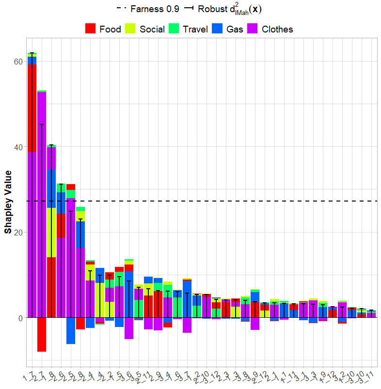
距離-距離プロットを作成し、外れ値を検出する:plot_dist_distコマンド
| オプション | 意味 | 初期値 |
|---|---|---|
| class_dist | 各観測値の古典的な距離。 | |
| class_cutoff | 古典的な距離のカットオフ値。 | NULL |
| class_cutoff_label | 古典的なカットオフの凡例ラベル。 | NULL |
| rob_dist | 各観測値のロバストな距離。 | |
| rob_cutoff | ロバストな距離のカットオフ値。 | NULL |
| rob_cutoff_label | ロバストカットオフのラベル。NULL(デフォルト)なら、ラベルが表示されない。 | NULL |
| obs_names | 観測値の名前を含む文字ベクトル。NULL(デフォルト)なら、class_distの名前を使用する。 | NULL |
| ggplotly | 論理値。TRUE(デフォルト)なら、プロットがインタラクティブなplotlyオブジェクトに変換される。 | TRUE |
| color_class | 各観測値の色クラスを示すベクトル。NULL(デフォルト)なら、すべての点が同じ色になる。 | NULL |
| color_label | 色クラスのラベル。NULL(デフォルト)なら、ラベルが表示されない。 | NULL |
| palette | 各色クラスの色を含むベクトル。NULL(デフォルト)なら、デフォルトのggplot2の色を使用する。 | NULL |
| shape_class | 各観測値の形状クラスを示すベクトル。NULL(デフォルト)なら、すべての点が同じ形状になる。 | NULL |
| shape_label | 形状クラスのラベル。NULL(デフォルト)なら、ラベルが表示されない。 | NULL |
| label_obs | ggplotly = FALSEの場合にプロットに表示される観測値の名前を含むベクトル。デフォルトはNULL。 | NULL |
# creditcardデータセットを読み込む
data(creditcard)
# intDataオブジェクトを作成
credit_card_int <- creditcard$intData
# ロバストな距離を計算
credit_card_dist <- IMah_dist(credit_card_int)
# 外れ値を検出
credit_card_outliers <- int_outliers(credit_card_dist,
                                     cutoff = "farness",
                                     cutoff_lvl = 0.9)
# 古典的な距離を計算
class_dist <- IMah_dist(credit_card_int, z = rep(1,credit_card_int@NObs))
# 古典的な外れ値を検出
class_outliers <- int_outliers(class_dist,
                               cutoff = "chi-squared",
                               p = credit_card_int@NIVar)
# 外れ値かどうかを示すラベル(Outlier/Inlier)を作成
credit_card_is_outliers <- as.character(credit_card_outliers$is_outlier)
credit_card_is_outliers[credit_card_outliers$is_outlier] <- "Outlier"
credit_card_is_outliers[!credit_card_outliers$is_outlier] <- "Inlier"
# 距離-距離プロットを表示
plot_dist_dist(class_dist,
               class_cutoff = class_outliers$cutoff_value,
               class_cutoff_label = "0.975 chi-squared",
               rob_dist = credit_card_dist,
               rob_cutoff = credit_card_outliers$cutoff_value,
               rob_cutoff_label = "0.9 farness",
               color_class = credit_card_is_outliers,
               palette = c("grey50", "red"))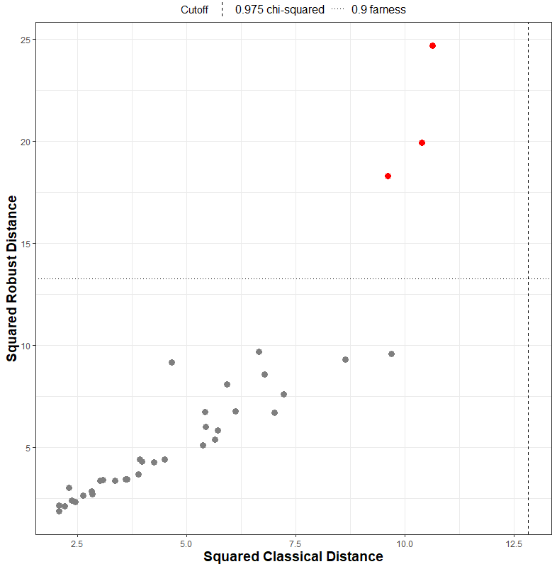
Shapley相互作用指標をプロット:plot_int_Shapley_interコマンド
| オプション | 意味 | 初期値 |
|---|---|---|
| x | 単一の観測値のShapley相互作用指標を含むp x p行列。 | |
| abbrev | 変数名を短縮する文字数の最小値 | 10 |
| title | プロットのタイトル | NULL |
| legend | 凡例を表示するかどうか | TRUE |
| text_size | プロット内のテキストサイズ | 22 |
# creditcardデータセットを読み込む
data(creditcard)
# intDataオブジェクトを作成
credit_card_int <- creditcard$intData
# ロバストなIMCD推定を取得
credit_card_IMCD <- IMCD(credit_card_int,
                         m = floor(nrow(credit_card_int)*0.75),
                         cutoff = "farness",
                         cutoff_lvl = 0.9)
# Shapley相互作用指標を計算
credit_card_shap_inter <- int_Shapley_interaction(credit_card_int,
                                                  mean_c = credit_card_IMCD$mean_IMCD_c,
                                                  mean_r = credit_card_IMCD$mean_IMCD_r,
                                                  cov = credit_card_IMCD$cov_IMCD)
# 1つ目の観測値のShapley相互作用をプロット
plot_int_Shapley_inter(credit_card_shap_inter[[1]])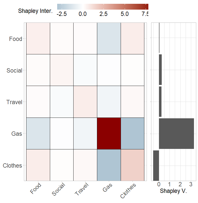

この記事が誰かの役に立ちますように。