Although it cannot accurately capture numerical values, the word cloud, also known as tag cloud, is an expression that strongly appeals to the sense of “characteristics of data by text”. Recently, we see it not only in the field of text mining such as search keywords and Twitter content, but also in omics analysis such as gene and metabolome.
Therefore, we introduce the “wordcloud” package, which makes it easy to create a word cloud.
Package version is 2.6. Checked with R version 4.2.2.
Install Package
Running the following command will install the RColorBrewer package, at the same time.
#Install Package
install.packages("wordcloud")
Command List
This is a list of commands available in the WordCloud package. For each command, options such as “xlab” and “ylb” of the plot command can be used.
| Type | Details | Command | Supplement |
|---|---|---|---|
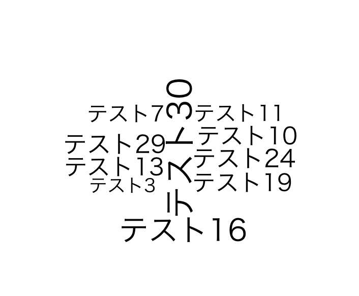
| Plot | Words that occur frequently between groups are displayed in order of decreasing difference in frequency between groups. | commonality.cloud(term.matrix, max.words = 300) | max.words:Specifies the number of words to display from the data. |
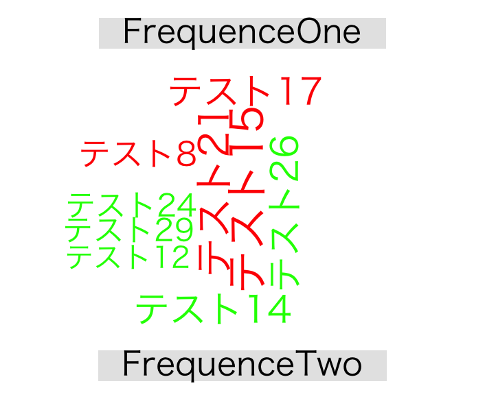
| Plot | Words that occur only in a particular group are given the highest priority, and words are displayed in group color in order of the number of occurrences per group and the smallest difference in frequency between groups. | comparison.cloud(term.matrix, scale = c(4,.5), max.words=300, random.order = FALSE, rot.per = .1, colors = brewer.pal(ncol(term.matrix), "Dark2"), use.r.layout = FALSE, title.size = 3) | omparing the two groups will plot the data, but will display a message about the COLORS setting. If you are concerned about this, please specify the COLORS setting. Example: c("red", "blue") |
| Data | The content of the union's speech. | data(SOTU) | List format. |
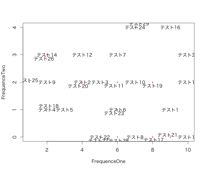
| Plot | Plots text on x- and y-axis coordinate data without overlapping. | textplot(x, y, words, cex = 1, new = TRUE, show.lines = TRUE) | |
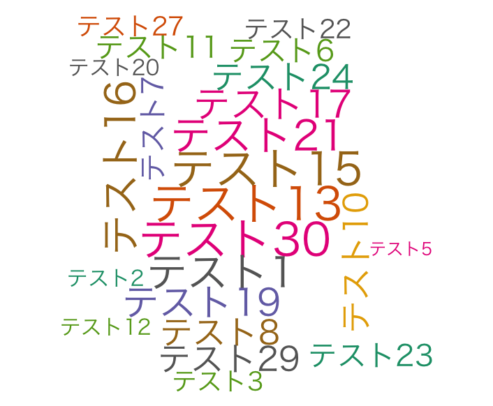
| Plot | Plot a word cloud. | wordcloud(words, freq, scale = c(4,.5), min.freq = 3, max.words = Inf, random.order = TRUE, random.color = FALSE, rot.per = .1, colors = "black", ordered.colors = FALSE, use.r.layout = FALSE, fixed.asp = TRUE) | scale:Set by array. c(size of characters, spacing between characters). random.order:If FALSE, plot words in order of highest frequency. min.freq:Minimum number of words to plot. random.color:If FALSE, colors are plotted in descending order. If order.colors:TRUE, colors are given in the order of the words. |
| Calculation | To avoid data overlap, the text plot coordinates are calculated and output in a matrix. | wordlayout(x, y, words, cex = 1, rotate90 = FALSE, xlim = c(-Inf,Inf), ylim = c(-Inf,Inf), tstep = .1, rstep = .1) | The result can be assigned to an argument. |
Example
See the command and package help for details.
#Loading the library
library("wordcloud")
#Creating Data
TestData <- data.frame(FrequenceOne = sample(1:10, 30, replace = TRUE),
FrequenceTwo = sample(0:4, 30, replace = TRUE),
row.names = paste("テスト", 1:30, sep = ""))
#commonality.cloud command
commonality.cloud(TestData, max.words = 10, random.order = FALSE)
#comparison.cloud command
comparison.cloud(TestData, max.words = 9, colors = c("red", "green"), random.order = FALSE)
#textplot command
textplot(TestData[,1], TestData[,2], rownames(TestData),
xlab = "FrequenceOne", ylab = "FrequenceTwo")
#wordcloud command
wordcloud(rownames(TestData), TestData[,1], scale = c(3, .5),
random.order = FALSE, rot.per = .1, random.color = TRUE, colors = brewer.pal(8, "Dark2"))
#wordlayout command
wordlayout(TestData[,1], TestData[,2], rownames(TestData))Output Example
commonality.cloud command
comparison.cloud command
textplot command
wordcloud command
I hope this makes your analysis a little easier !!