Analysis in R: Presented in R MarkDown! A lot of color palette “ggsci” package

This is an introduction to a package that contains a color palette that can also be used with ggplot2. The color palette can be verified by running the rmd file in the command introduction.

The package version is 2.9. Tested with R version 4.2.2.

Install Package

Run the following command.

#Install Package
install.packages("ggsci")

Example

See the command and package help for details.You can download the file below and run it in RStudio to get the same results as the introduction of the same command. The file extension is Rmd.

ggsci.Rmd

1 file(s) 4.09 KB

Download

---
title: "ggsci"
output:
  flexdashboard::flex_dashboard:
  orientation: columns
social: menu
source_code: embed
runtime: shiny
---
  
  ```{r global, include=FALSE}
#Loading the library
if(!require("ggsci", quietly = TRUE)){
  install.packages("ggsci");require("ggsci")
}
if(!require("tidyverse", quietly = TRUE)){
  install.packages("tidyverse");require("tidyverse")
}
if(!require("flexdashboard", quietly = TRUE)){
  install.packages("flexdashboard");require("flexdashboard")
}
if(!require("DT", quietly = TRUE)){
  install.packages("DT");require("DT")
}

###Creating Data#####
n <- 100
TestData <- data.frame("Group" = sample(paste0("Group", 1:5), n, replace = TRUE),
                          "Data1" = sample(1:10, n, replace = TRUE),
                          "Data2" = sample(LETTERS[1:24], n, replace = TRUE))
########
#「ggsci」pakage:Color Palettes Name
GgSColName <- c("AAAS Journal Color Palettes", "D3.js Color Palettes", "The Futurama Color Palettes",
                   "Integrative Genomics Viewer (IGV) Color Palettes", "Journal of Clinical Oncology Color Palettes",
                   "Lancet Journal Color Palettes", "LocusZoom Color Palette", "NEJM Color Palettes",
                   "NPG Journal Color Palettes", "Rick and Morty Color Palettes", "The Simpsons Color Palettes",
                   "Star Trek Color Palettes", "The University of Chicago Color Palettes",
                   "UCSC Genome Browser Color Palette")

#"ggsci" package: Symbol color commands available in ggplot2
GgScalCol <- c("scale_color_aaas()", "scale_color_d3()", "scale_color_futurama()",
                  "scale_color_igv()", "scale_color_jco()", "scale_color_lancet()",
                  "scale_color_locuszoom()", "scale_color_nejm()", "scale_color_npg()",
                  "scale_color_rickandmorty()", "scale_color_simpsons()", "scale_color_startrek()",
                  "scale_color_uchicago()", "scale_color_ucscgb()")
#「ggsci」パッケージ:ggplot2で使える塗色コマンド
GgScalFill <- c("scale_fill_aaas()", "scale_fill_d3()", "scale_fill_futurama()",
                   "scale_fill_igv()", "scale_fill_jco()", "scale_fill_lancet()",
                   "scale_fill_locuszoom()", "scale_fill_nejm()", "scale_fill_npg()",
                   "scale_fill_rickandmorty()", "scale_fill_simpsons()", "scale_fill_startrek()",
                   "scale_fill_uchicago()", "scale_fill_ucscgb()")

#"ggsci" package: Included color palette commands
GgScalPal <- c("pal_aaas()", "pal_d3()", "pal_futurama()",
                  "pal_igv()", "pal_jco()", "pal_lancet()",
                  "pal_locuszoom()", "pal_nejm()", "pal_npg()",
                  "pal_rickandmorty()", "pal_simpsons()", "pal_startrek()",
                  "pal_uchicago()", "pal_ucscgb()")

#"ggsci" package:Number of colors in each color palette included
GgScalNO <- c(10, 10, 12, 51, 10, 9, 7, 8, 10, 12, 16, 7, 9, 26)
```

Column {data-width=500}
-------------------------------------
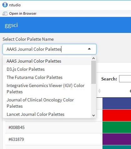
  ```{r}
selectInput('Colpal', 'Select Color Palette Name', GgSColName)

```

###Included Color Palette

```{r}
renderDataTable({
  ColCodeData <- eval(parse(text = paste0(GgScalPal[which(GgSColName == input$Colpal)], "(", GgScalNO[which(GgSColName == input$Colpal)], ")")))
  ColCodeData <- data.frame("ColerCode" = strtrim(ColCodeData, 7),
                               "Color" = rep("", length(ColCodeData)))
  datatable(ColCodeData, rownames = FALSE,
            options = list(pageLength = 10, lengthMenu = c(20, 40, 100))) %>%
    formatStyle("Color", valueColumns = "ColerCode",
                backgroundColor = styleEqual(ColCodeData[, 1], ColCodeData[, 1]))
})
```

Column {data-width=500}
-------------------------------------
  
  ###Color
  ```{r}
renderPlot({
  ggplot(TestData,
         aes(x = Data1, y = Data2, col = Group)) +
    geom_point(size = 10) +
    theme_bw() +
    eval(parse(text = GgScalCol[which(GgSColName == input$Colpal)])) +
    labs(title = paste0(GgScalCol[which(GgSColName == input$Colpal)], " コマンド"))
})
```

###Fill
```{r}
renderPlot({
  ggplot(TestData,
         aes(x = Data2, fill = Group)) +
    geom_histogram(stat = "count") +
    
    
    theme_bw() +
    eval(parse(text = GgScalFill[which(GgSColName == input$Colpal)])) +
    labs(title = paste0(GgScalFill[which(GgSColName == input$Colpal)], " コマンド"))
})
```

Output Example

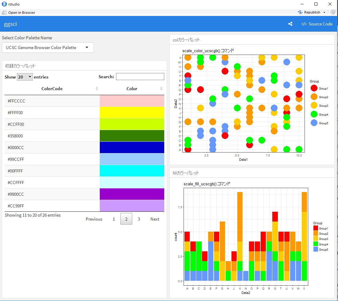
I hope this makes your analysis a little easier !!