Rで解析：EMF/EMF+ファイルの作成「devEMF」パッケージ

プロットをWindowsでおなじみの「EMF」ファイルまたは「EMF+」ファイルで出力可能なパッケージの紹介です。パッケージ収録の「emf」コマンドと「dev.off」コマンドの間にプロットコマンドを記述するだけで出力できます。

簡単にファイルサイズが小さく綺麗な画像を出力でき、Microsoft OfficeやLibreOfficeで利用することが可能です。

パッケージバージョンは4.1-2。windows11のR version 4.2.2で確認しています。

パッケージのインストール

下記コマンドを実行してください。

#&#12497;&#12483;&#12465;&#12540;&#12472;&#12398;&#12452;&#12531;&#12473;&#12488;&#12540;&#12523;
install.packages("devEMF")

実行コマンド

詳細はコマンド、パッケージのヘルプを確認してください。図は「ggtrace」パッケージを利用してプロットしました。

#&#12497;&#12483;&#12465;&#12540;&#12472;&#12398;&#35501;&#12415;&#36796;&#12415;
library("devEMF")

#EMF&#12501;&#12449;&#12452;&#12523;&#12398;&#20316;&#25104;:emf&#12467;&#12510;&#12531;&#12489;;dev.off&#12467;&#12510;&#12531;&#12489;&#12392;&#32068;&#12415;&#21512;&#12431;&#12379;&#12390;&#20351;&#29992;&#12375;&#12414;&#12377;
#&#20986;&#21147;&#12501;&#12449;&#12452;&#12523;&#21517;:file&#12458;&#12503;&#12471;&#12519;&#12531;
#&#24133;,&#39640;:width/height&#12458;&#12503;&#12471;&#12519;&#12531;
#&#24133;,&#39640;&#12398;&#21336;&#20301;:units&#12458;&#12503;&#12471;&#12519;&#12531;;"in","cm","mm"
#&#12521;&#12505;&#12523;&#31561;&#12398;&#12501;&#12457;&#12531;&#12488;&#12469;&#12452;&#12474;:pointsize&#12458;&#12503;&#12471;&#12519;&#12531;
#&#21508;&#31278;EMF+&#12501;&#12449;&#12452;&#12523;&#12398;&#35373;&#23450;:
#emfPlus/emfPlusFont/emfPlusRaster/emfPlusFontToPath&#12458;&#12503;&#12471;&#12519;&#12531;
#LibreOffice&#12395;&#36969;&#24540;&#12377;&#12427;EMF&#12501;&#12449;&#12452;&#12523;&#12399;:emfPlus&#12458;&#12503;&#12471;&#12519;&#12531;&#12434;TRUE&#12395;&#12377;&#12427;
emf(file = "&#20986;&#21147;&#12501;&#12449;&#12452;&#12523;&#21517;", 
    width = 7, height = 7,
    units = "cm", pointsize = 12, 
    emfPlus = TRUE, emfPlusFont = FALSE,
    emfPlusRaster = FALSE, emfPlusFontToPath = FALSE)

###########################
###emf&#12467;&#12510;&#12531;&#12489;&#12398;&#20181;&#27096;&#20363;#####
###########################
###&#12487;&#12540;&#12479;&#20363;&#12398;&#20316;&#25104;#####
#tidyverse&#12497;&#12483;&#12465;&#12540;&#12472;&#12364;&#12394;&#12369;&#12428;&#12400;&#12452;&#12531;&#12473;&#12488;&#12540;&#12523;
if(!require("tidyverse", quietly = TRUE)){
  install.packages("tidyverse");require("tidyverse")
}
#&#20081;&#25968;&#12398;&#22266;&#23450;
set.seed(1234)
n <- 30
GName <- paste0("Group", 1:3)
TestData <- tibble(Group = rep(GName, each = n),
                   Day = rep(1:n, time = length(GName)),
                   X = sample(c(1:50), n*length(GName), replace = TRUE),
                   Y = sample(c(51:100), n*length(GName), replace = TRUE))
########

#&#12300;ggtrace&#12301;&#12497;&#12483;&#12465;&#12540;&#12472;&#12434;&#21033;&#29992;&#12375;&#12390;&#12503;&#12525;&#12483;&#12488;
#https://www.karada-good.net/analyticsr/r-737/
#ggtrace&#12497;&#12483;&#12465;&#12540;&#12472;&#12364;&#12394;&#12369;&#12428;&#12400;&#12452;&#12531;&#12473;&#12488;&#12540;&#12523;
if(!require("ggtrace", quietly = TRUE)){
  install.packages("ggtrace");require("ggtrace")
}
#StepPlot&#12398;&#12450;&#12454;&#12488;&#12521;&#12452;&#12531;&#12392;&#12495;&#12452;&#12521;&#12452;&#12488;&#12434;&#20316;&#25104;:geom_step_trace&#12467;&#12510;&#12531;&#12489;
TestPlot <- ggplot(TestData, aes(x = Day, y = Y, fill = Group)) +
  #geom_step_trace&#12467;&#12510;&#12531;&#12489;
  #&#12458;&#12503;&#12471;&#12519;&#12531;&#12399;geom_line_trace&#12467;&#12510;&#12531;&#12489;&#12392;&#20849;&#36890;
  geom_step_trace(
    trace_position = Day <= 10 | Day >= 20,
    background_params = list(color = "red", fill = "grey75",
                             size = 1, stroke = 0.5,
                             linetype = 1, alpha = 0.5),
    color = "#4b61ba", size = 1, stroke = 1,
    linetype = 1, alpha = 1) +
  theme(plot.background = element_rect(fill = "black"),
        panel.background = element_rect(fill = "black"),
        axis.text = element_text(colour = "white"))
########

###&#20316;&#26989;&#12501;&#12457;&#12523;&#12480;&#12395;EMF&#12501;&#12449;&#12452;&#12523;&#12434;&#20986;&#21147;#####
emf("TestGGplot.emf")
#emf&#12467;&#12510;&#12531;&#12489;&#12392;dev.off&#12467;&#12510;&#12531;&#12489;&#12398;&#38291;&#12395;&#12503;&#12525;&#12483;&#12488;&#12467;&#12510;&#12531;&#12489;&#12434;&#35352;&#36848;&#12377;&#12427;
TestPlot
dev.off()
########

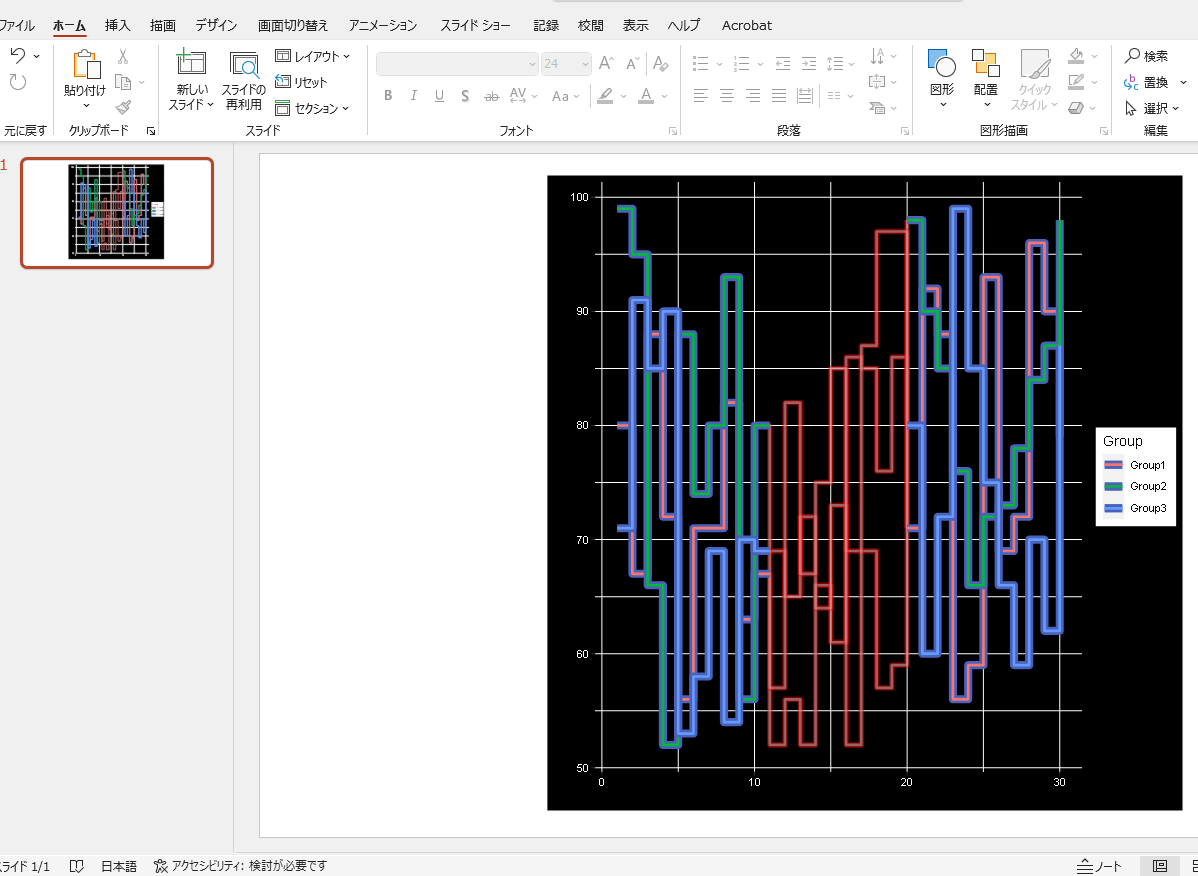
出力例

出力をPowerPointに張り付けた例です。

少しでも、あなたの解析が楽になりますように！！