Rで解析：ベーシックなカラーパレットです「colorRamps」パッケージ

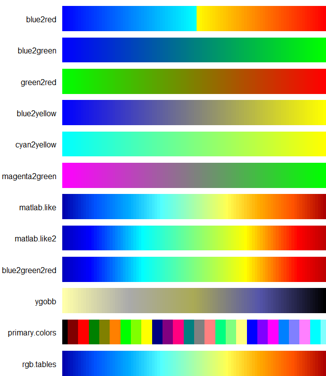
使いやすいカラーパレットが収録されているパッケージの紹介です。12のカラーパレットが収録されています。「colorRamps」は2007年から更新が続いているパッケージです。ベーシックなカラーパレットは使い勝手がいいと思います。

バージョンは2.3.1。実行コマンドはwindows 11のR version 4.1.3で確認しています。

パッケージのインストール

下記コマンドを実行してください。

#パッケージのインストール
install.packages("colorRamps")

実行コマンド

詳細はコメント、パッケージヘルプを確認してください。

#パッケージの読み込み
library("colorRamps")

##プロット準備
par(mfrow = c(12, 1), mar = c(0, 10, 1, 0))
n <- 100
########

#各カラーパレットのコマンド実行
for(i in 1:12){
  
  #blue2red
  image(1:n, 1, matrix(1:n, n), lwd = 2,
        col = blue2red(n), axes = FALSE,
        xlab = "", ylab = "",)
  mtext("blue2red", line = 1, srt = -45,
        side = 2, cex.lab = 1, las = 2)  
  #blue2green
  image(1:n, 1, matrix(1:n, n),
        col = blue2green(n), axes = FALSE,
        xlab = "", ylab = "")
  mtext("blue2green", line = 1, srt = -45,
        side = 2, cex.lab = 1, las = 2)  
  #green2red
  image(1:n, 1, matrix(1:n, n),
        col = green2red(n), axes = FALSE,
        xlab = "", ylab = "")
  mtext("green2red", line = 1, srt = -45,
        side = 2, cex.lab = 1, las = 2) 
  #blue2yellow
  image(1:n, 1, matrix(1:n, n),
        col = blue2yellow(n), axes = FALSE,
        xlab = "", ylab = "")
  mtext("blue2yellow", line = 1, srt = -45,
        side = 2, cex.lab = 1, las = 2) 
  #cyan2yellow
  image(1:n, 1, matrix(1:n, n),
        col = cyan2yellow(n), axes = FALSE,
        xlab = "", ylab = "")
  mtext("cyan2yellow", line = 1, srt = -45,
        side = 2, cex.lab = 1, las = 2) 
  #magenta2green
  image(1:n, 1, matrix(1:n, n),
        col = magenta2green(n), axes = FALSE,
        xlab = "", ylab = "")
  mtext("magenta2green", line = 1, srt = -45,
        side = 2, cex.lab = 1, las = 2) 
  #matlab.like
  image(1:n, 1, matrix(1:n, n),
        col = matlab.like(n), axes = FALSE,
        xlab = "", ylab = "")
  mtext("matlab.like", line = 1, srt = -45,
        side = 2, cex.lab = 1, las = 2) 
  #matlab.like2
  image(1:n, 1, matrix(1:n, n),
        col = matlab.like2(n), axes = FALSE,
        xlab = "", ylab = "")
  mtext("matlab.like2", line = 1, srt = -45,
        side = 2, cex.lab = 1, las = 2) 
  #blue2green2red
  image(1:n, 1, matrix(1:n, n),
        col = blue2green2red(n), axes = FALSE,
        xlab = "", ylab = "")
  mtext("blue2green2red", line = 1, srt = -45,
        side = 2, cex.lab = 1, las = 2)
  #ygobb
  image(1:n, 1, matrix(1:n, n),
        col = ygobb(n), axes = FALSE,
        xlab = "", ylab = "")
  mtext("ygobb", line = 1, srt = -45,
        side = 2, cex.lab = 1, las = 2)
  #primary.colors
  image(1:n, 1, matrix(1:n, n),
        col = primary.colors(100), axes = FALSE,
        xlab = "", ylab = "")
  mtext("primary.colors", line = 1, srt = -45,
        side = 2, cex.lab = 1, las = 2)
  #rgb.tables
  image(1:n, 1, matrix(1:n, n),
        col = rgb.tables(n = n,
                         red = c(0.75, 0.25, 1),
                         green = c(0.5, 0.25, 1),
                         blue = c(0.25, 0.25, 1)), axes = FALSE,
        xlab = "", ylab = "")
  mtext("rgb.tables", line = 1, srt = -45,
        side = 2, cex.lab = 1, las = 2)
}

出力例

少しでも、あなたの解析が楽になりますように！！