Rで解析：Sankey Plotに便利です「sankey」パッケージ

作業フローやKPIなどの描写に便利なSankey PlotやSankey Diagramと呼ばれる手法があります。データの準備に癖があるかもしれませんが有用な表現方法だと思います。

プロット体裁に必要な情報は表でまとめていますので参考にしてください。

パッケージバージョンは1.0.2。windows11のR version 4.2.2で確認しています。

＜おすすめのRに関する書籍です＞

東京大学のデータサイエンティスト育成講座 ~Pythonで手を動かして学ぶデ―タ分析~ | 塚本邦尊, 山田典一, 大澤文孝, 中山浩太郎, 松尾 豊[協力]

Amazonで塚本邦尊, 山田典一, 大澤文孝, 中山浩太郎, 松尾 豊[協力]の東京大学のデータサイエンティスト育成講座 ~Pythonで手を動かして学ぶデ―タ分析~。アマゾンならポイント還元本が多数。

www.amazon.co.jp

パッケージのインストール

下記、コマンドを実行してください。

#パッケージのインストール
install.packages("sankey")

実行コマンド

詳細はコメント、パッケージのヘルプを確認してください。

#パッケージの読み込み
library("sankey")

###データ例の作成#####
n <- 15
#結合データを用意
#同じ長さの2つの配列
V1 <- sample(letters[1:24], n, replace = TRUE)
V2 <- sample(letters[1:24], n, replace = TRUE)

#配列からグラフ用のデータを作成
GraphText <- NULL
for(i in seq(V1)){

  GraphText <- paste(GraphText, V1[i], V2[i], "\n", sep = " ")

}
########

#edge読み込みデータの作成
edges <- read.table(stringsAsFactors = FALSE, textConnection(GraphText))

#edgeデータの作成:make_sankeyコマンド
PlotEdgeData <- make_sankey(edges = edges)
#構造の確認
str(PlotEdgeData)
List of 2
$ nodes:'data.frame':	16 obs. of  19 variables:
..$ id     : chr [1:16] "a" "t" "p" "v" ...
..$ col    : chr [1:16] "#2ca25f" "#2ca25f" "#2ca25f" "#2ca25f" ...
..$ shape  : chr [1:16] "rectangle" "rectangle" "rectangle" "rectangle" ...
..$ lty    : num [1:16] 1 1 1 1 1 1 1 1 1 1 ...
..$ srt    : num [1:16] 0 0 0 0 0 0 0 0 0 0 ...
..$ textcol: chr [1:16] "black" "black" "black" "black" ...
..$ label  : chr [1:16] "a" "t" "p" "v" ...
..$ adjx   : num [1:16] 0.5 0.5 0.5 0.5 0.5 0.5 0.5 0.5 0.5 0.5 ...
..$ adjy   : num [1:16] 1 1 1 1 1 1 1 1 1 1 ...
..$ boxw   : num [1:16] 0.2 0.2 0.2 0.2 0.2 0.2 0.2 0.2 0.2 0.2 ...
..$ cex    : num [1:16] 0.7 0.7 0.7 0.7 0.7 0.7 0.7 0.7 0.7 0.7 ...
..$ size   : num [1:16] 2 1 1 3 2 1 2 1 1 2 ...
..$ x      : num [1:16] 0 0 0 0 0 1 1 1 1 1 ...
..$ bottom : num [1:16] -1.35 -6.05 -9.75 -13.45 -19.15 ...
..$ top    : num [1:16] -3.35 -7.05 -10.75 -16.45 -21.15 ...
..$ center : num [1:16] -2.35 -6.55 -10.25 -14.95 -20.15 ...
..$ pos    : num [1:16] 2 2 2 2 2 1 1 1 1 1 ...
..$ textx  : num [1:16] -0.1 -0.1 -0.1 -0.1 -0.1 1 1 1 1 1 ...
..$ texty  : num [1:16] -2.35 -6.55 -10.25 -14.95 -20.15 ...
$ edges:'data.frame':	15 obs. of  6 variables:
..$ V1        : chr [1:15] "w" "w" "v" "v" ...
..$ V2        : chr [1:15] "e" "c" "c" "l" ...
..$ colorstyle: chr [1:15] "gradient" "gradient" "gradient" "gradient" ...
..$ curvestyle: chr [1:15] "sin" "sin" "sin" "sin" ...
..$ col       : chr [1:15] "#99d8c9" "#99d8c9" "#99d8c9" "#99d8c9" ...
..$ weight    : num [1:15] 1 1 1 1 1 1 1 1 1 1 ...
- attr(*, "class")= chr [1:3] "sankey" "simplegraph_df" "simplegraph"

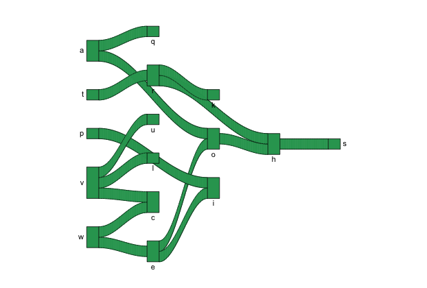
#プロット:sankeyコマンド
sankey(PlotEdgeData)

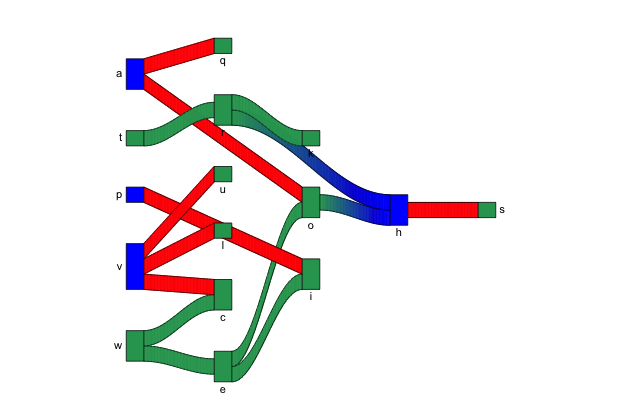
###グラフ体裁はedgeデータ内容を変更します########
#ノードの色を変更
PlotEdgeData$nodes$col <- ifelse(PlotEdgeData$nodes$id %in% c("a", "p", "v", "h"), "blue", "#2ca25f")
#エッジの色を変更
PlotEdgeData$edges$col <- ifelse(PlotEdgeData$edges$V1 %in% c("a", "p", "v", "h"), "red", "yellow")
#エッジの塗りつぶし方法を変更
PlotEdgeData$edges$colorstyle <- ifelse(PlotEdgeData$edges$V1 %in% c("a", "p", "v", "h"), "col", "gradient")
#エッジの塗りつぶし方法を変更
PlotEdgeData$edges$curvestyle <- ifelse(PlotEdgeData$edges$V1 %in% c("a", "p", "v", "h"), "line", "sin")
#プロット
sankey(PlotEdgeData)

プロット体裁に必要な情報

出力例

・sankeyコマンド

・体裁を変更してプロット

少しでも、あなたの解析が楽になりますように！！

＜おすすめのRに関する書籍です＞

初心者でもすぐにできるフリー統計ソフトEZR(Easy R)で誰でも簡単統計解析(改訂第2版) | 神田善伸

Amazonで神田善伸の初心者でもすぐにできるフリー統計ソフトEZR(Easy R)で誰でも簡単統計解析(改訂第2版)。アマゾンならポイント還元本が多数。

www.amazon.co.jp