Rで解析：ggplot2の体裁に役に立つかも？「ggthemes」パッケージ

公開日 2023-01-15

Rの解析に役に立つ記事

ggplot2の体裁を整えるのに役に立つかもしれないパッケージの紹介です。テーマやカラーパレット、塗りパレットなどが収録されています。

パッケージバージョンは4.2.4。R version 4.2.2で確認しています。

＜おすすめのRに関する書籍です＞

改訂3版 R言語逆引きハンドブック | 石田基広

Amazonで石田基広の改訂3版 R言語逆引きハンドブック。アマゾンならポイント還元本が多数。石田基広作品ほか、お急ぎ便対象商品は当日お届けも可能。また改訂3版 R言語逆引きハンドブックもアマゾン配送商品なら通常配送無料。

www.amazon.co.jp

パッケージのインストール

下記コマンドを実行してください。

#パッケージのインストール
install.packages("ggthemes")

コマンドの紹介

詳細はコマンド、各パッケージのヘルプを確認してください。

#パッケージの読み込み
library("ggthemes")

###データ例の作成#####
#ggplot2を利用するためにtidyverseパッケージ
#tidyverseパッケージがなければインストール
if(!require("tidyverse", quietly = TRUE)){
  install.packages("tidyverse");require("tidyverse")
}

n <- 150
TestData <- data.frame("Group" = sample(paste0("Group", 1:5), n, replace = TRUE),
                       "x" = sample(c(1:100), n, replace = TRUE),
                       "y" = sample(c(1:200), n, replace = TRUE),
                       "LETTERS" = sample(LETTERS[1:24], n, replace = TRUE))

########

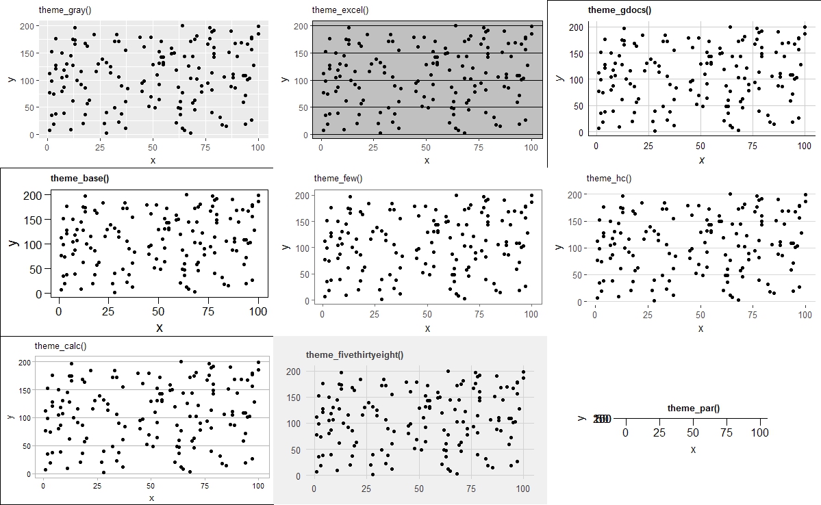
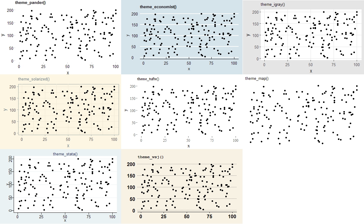
#ggthemesパッケージに収録されているテーマを適用
#テーマを設定,theme_gray()はggplot2の初期値
Theme <- c("theme_gray()", "theme_base()", "theme_calc()",
           "theme_excel()", "theme_few()", "theme_fivethirtyeight()",
           "theme_gdocs()", "theme_hc()", "theme_par()",
           "theme_pander()", "theme_solarized()", "theme_stata()",
           "theme_economist()","theme_tufte()", "theme_wsj()",
           "theme_igray()", "theme_map()")
#画面分割のためgridパッケージを利用
library("grid")
#新規プロットエリア
grid.newpage()
#3行3列
pushViewport(viewport(layout = grid.layout(3, 3)))
#プロット場所指定の変数を用意
Xpos <- rep(1:3, times = 6)
Ypos <- rep(1:3, each = 3, length = 18)
#プロット
for(i in seq(Theme)){
  if(i == 10) {
    grid.newpage()
    pushViewport(viewport(layout = grid.layout(3, 3)))}

  print(ggplot(TestData, aes(x = x, y = y)) +
          geom_point() +
          eval(parse(text = Theme[i])) +
          labs(title = Theme[i]) +
          theme(plot.title = element_text(size = 10)),
        vp = viewport(layout.pos.row = Xpos[i], layout.pos.col = Ypos[i]))}

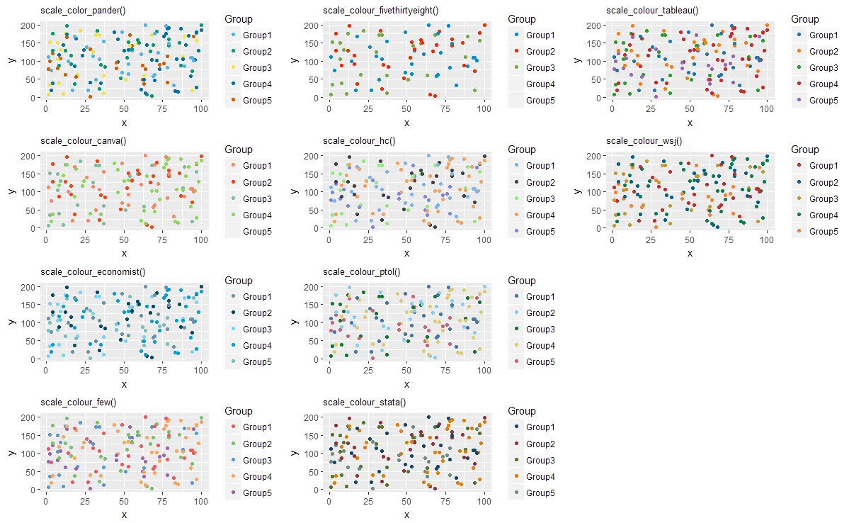
#ggthemesパッケージに収録されているカラーテーマを適用
ColTheme <- c("scale_color_pander()", "scale_colour_canva()", "scale_colour_economist()",
              "scale_colour_few()", "scale_colour_fivethirtyeight()", "scale_colour_hc()",
              "scale_colour_ptol()", "scale_colour_stata()", "scale_colour_tableau()",
              "scale_colour_wsj()")
#画面分割のためgridパッケージを利用
library("grid")
#新規プロットエリア
grid.newpage()
#4行3列
pushViewport(viewport(layout = grid.layout(4, 3)))
#プロット場所指定の変数を用意
Xpos <- rep(1:4, times = 3)
Ypos <- rep(1:3, each = 4, length = 12)
#プロット
for(i in seq(ColTheme)){
  print(ggplot(TestData, aes(x = x, y = y, col = Group)) +
          geom_point() +
          eval(parse(text = ColTheme[i])) +
          labs(title = ColTheme[i]) +
          theme(plot.title = element_text(size = 10)),
        vp = viewport(layout.pos.row = Xpos[i], layout.pos.col = Ypos[i]))}

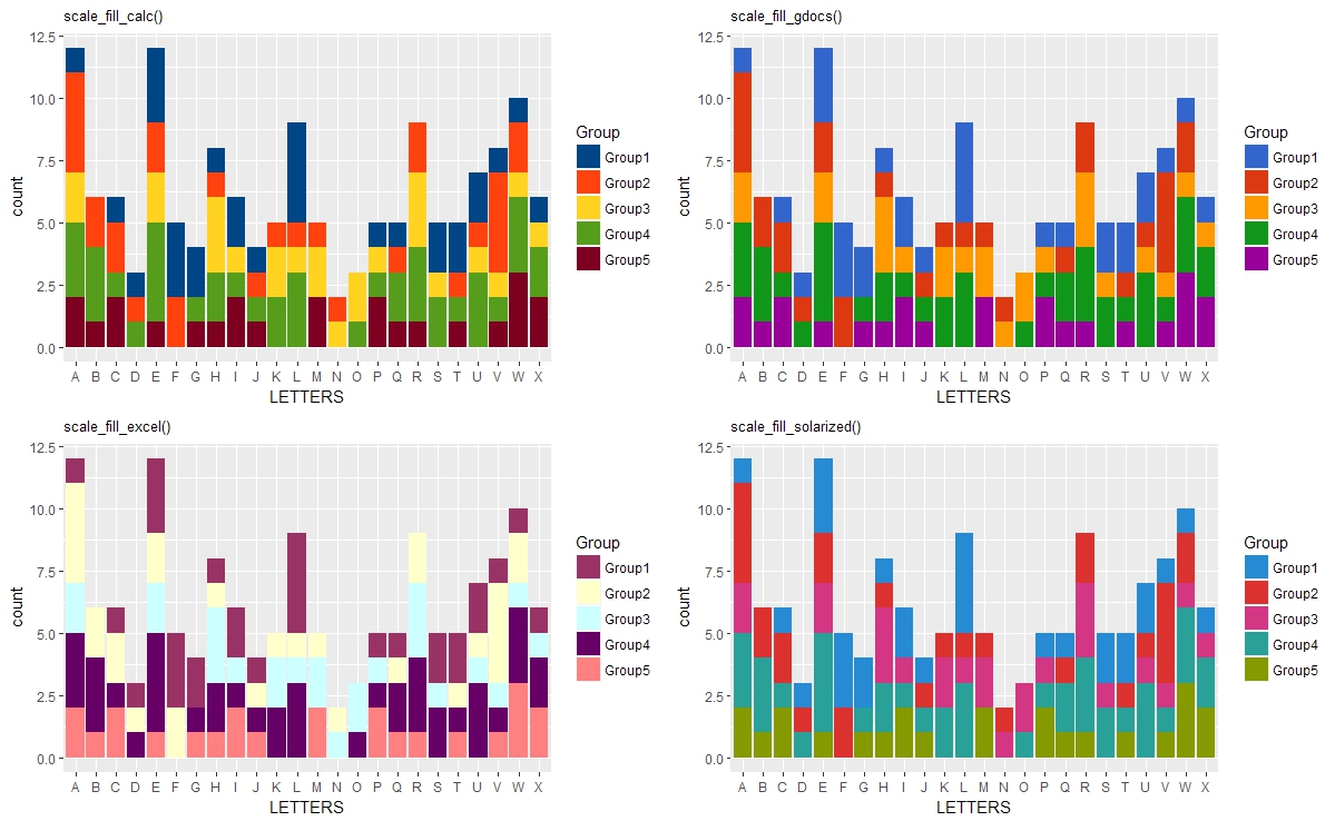
#ggthemesパッケージに収録されている塗テーマを適用
FillTheme <- c("scale_fill_calc()", "scale_fill_excel()",
               "scale_fill_gdocs()", "scale_fill_solarized()")
#画面分割のためgridパッケージを利用
library("grid")
#新規プロットエリア
grid.newpage()
#2行2列
pushViewport(viewport(layout = grid.layout(2, 2)))
#プロット場所指定の変数を用意
Xpos <- c(1, 2, 1, 2)
Ypos <- c(1, 1, 2, 2)
#プロット
for(i in seq(FillTheme)){
  print(ggplot(TestData, aes(x = LETTERS, fill = Group)) +
          geom_histogram(stat = "count") +
          eval(parse(text = FillTheme[i])) +
          labs(title = FillTheme[i]) +
          theme(plot.title = element_text(size = 10)),
        vp = viewport(layout.pos.row = Xpos[i], layout.pos.col = Ypos[i]))}