市場調査や心理学などで使用されるレパートリー・グリッドを作成・解析するパッケージの紹介です。
レパートリー・グリッドを初めて聞きました。
どのようなデータが解析対象となるのか解らなかったので、下記論文のFig4のデータを参考にしています。
・阿部ひと美・今井正司・根建金男(2013)
レパートリー・グリッド法を適用してとらえた社会不安の特徴
パーソナリティ研究, 21, 203-215.
https://www.jstage.jst.go.jp/article/personality/21/3/21_203/_pdf
論文でも主張されていますが、レパートリー・グリッドは大変可能性があるツールだと考えます。
なお紹介していませんが、テキストファイルなどからレパートリー・グリッドのデータを読み込むコマンドがパッケージに収録されています。パッケージヘルプだけでなくOpenRepGrid公式ページも参考にしてください。
・OpenRepGrid公式ページ
http://docu.openrepgrid.org/index.html
パッケージバージョンは0.1.12。R version 4.2.2で動作を確認しています。
パッケージのインストール
下記コマンドを実行してください。
#パッケージのインストール
install.packages("OpenRepGrid")
コマンドの紹介
詳細はコマンド、各パッケージのヘルプを確認してください。
#パッケージの読み込み
library("OpenRepGrid")
#レパートリー・グリッドの作成とスケールの設定:makeRepgrid,setScaleコマンド
TestData <- list(
name = c("初対面の異性と話す", "初対面の同姓と話す",
"人前で発表する", "よく知らない人に電話をかける",
"グループの中で自分の意見を言う", "授業中に先生に質問をする",
"誰かを誘おうとする", "親しくない人に頼みごとをする",
"権威のある人と話す", "重要な試験を受ける",
"学食やレストランで食事をする", "友人に電話を掛ける",
"盛り上がって輪の中に入る", "親しくない人と話す",
"親しい友人と話す"),
l.name = c("緊張する", "自分がどう思われているか気になる",
"自信がない", "苦手である", "避けようとする",
"難しい", "消極的である", "態度がぎこちない",
"パニックになる", "頭が混乱する", "表情がこわばる",
"つまらない", "口ごもる", "言いたいことが言えない"),
r.name = c("リラックスする", "自分がどう思われようと気にしない",
"自信がある", "得意である", "進んで取り組む",
"たやすい", "積極的である", "自然な態度",
"落ち着いている", "頭がはっきりしている",
"表情が自然", "よくしゃべる", "楽しい",
"はきはきと話す", "言いたいことが言える"),
scores = c(1, 1, 1, 1, 2, 1, 1, 1, 3, 2, 5, 3, 3, 3, 6,
3, 3, 2, 4, 3, 3, 2, 3, 4, 4, 5, 3, 3, 2, 3,
2, 2, 3, 2, 3, 3, 2, 3, 4, 4, 4, 4, 2, 2, 4,
2, 2, 3, 1, 3, 2, 1, 3, 4, 4, 3, 3, 2, 3, 4,
4, 4, 2, 1, 2, 2, 2, 3, 3, 4, 4, 3, 3, 6, 6,
3, 3, 2, 2, 2, 2, 2, 3, 4, 3, 5, 3, 3, 3, 6,
3, 3, 3, 3, 3, 2, 2, 3, 1, 4, 4, 3, 3, 4, 6,
3, 3, 3, 2, 3, 3, 3, 2, 3, 4, 5, 5, 4, 4, 7,
3, 3, 2, 2, 3, 3, 3, 3, 3, 4, 4, 4, 4, 3, 7,
2, 2, 1, 3, 3, 3, 3, 3, 3, 6, 4, 5, 4, 3, 6,
1, 1, 2, 3, 3, 3, 4, 3, 3, 1, 4, 6, 6, 6, 7,
2, 2, 6, 4, 4, 5, 5, 5, 3, 1, 4, 6, 5, 4, 7,
4, 4, 4, 4, 4, 4, 4, 4, 4, 4, 5, 6, 6, 4, 7,
2, 2, 5, 5, 5, 3, 3, 6, 5, 4, 4, 6, 5, 6, 6,
2, 2, 7, 5, 5, 3, 3, 3, 2, 4, 4, 7, 4, 4, 6))
#グリッドの作成:makeRepgridコマンド
TestGrid <- makeRepgrid(TestData)
#スケールの設定:setScaleコマンド
TestGrid <- setScale(TestGrid, 1, 7)
#グリッドの表示
TestGrid
########
#グリッドデータの統計情報を表示:statsConstructsコマンド
#コンストラクトの文字表示数:trimオプション
#項目番号の表示:indexオプション
Result <- statsConstructs(TestGrid, trim = 10, index = TRUE)
#class確認
class(Result)
[1] "statsConstructs" "data.frame"
#結果を表示
Result
####################################
Desriptive statistics for constructs
####################################
vars n mean sd median trimmed mad min max range skew kurtosis se
(1) 緊張する - リラックス 1 15 2.27 1.58 2 2.08 1.48 1 6 5 1.01 -0.12 0.41
(2) 自分がどう - 自分がどう 2 15 3.13 0.83 3 3.08 0.00 2 5 3 0.47 -0.41 0.22
(3) 自信がない - 自信がある 3 15 2.93 0.88 3 2.92 1.48 2 4 2 0.12 -1.79 0.23
(4) 苦手である - 得意である 4 15 2.67 0.98 3 2.69 1.48 1 4 3 -0.22 -1.11 0.25
(5) 避けようと - 進んで取り 5 15 3.27 1.44 3 3.23 1.48 1 6 5 0.51 -0.67 0.37
(6) 難しい - たやすい 6 15 3.07 1.16 3 2.92 1.48 2 6 4 1.15 0.47 0.30
(7) 消極的であ - 積極的であ 7 15 3.13 1.13 3 3.08 0.00 1 6 5 0.60 0.87 0.29
(8) 態度がぎこ - 自然な態度 8 15 3.60 1.30 3 3.46 1.48 2 7 5 1.07 0.65 0.34
(9) パニックに - 落ち着いて 9 15 3.40 1.18 3 3.23 0.00 2 7 5 1.67 3.00 0.31
(10) 頭が混乱す - 頭がはっき 10 15 3.40 1.40 3 3.38 1.48 1 6 5 0.48 -0.61 0.36
(11) 表情がこわ - 表情が自然 11 15 3.53 1.96 3 3.46 1.48 1 7 6 0.30 -1.26 0.51
(12) つまらない - よくしゃべ 12 15 4.20 1.66 4 4.23 1.48 1 7 6 -0.30 -0.89 0.43
(13) 口ごもる - 楽しい 13 15 4.53 0.99 4 4.38 0.00 4 7 3 1.36 0.27 0.26
(14) 言いたいこ - はきはきと 14 15 4.47 1.41 5 4.54 1.48 2 6 4 -0.51 -1.20 0.36
(15) 緊張する - 言いたいこ 15 15 4.07 1.67 4 4.00 1.48 2 7 5 0.42 -1.08 0.43
#コンストラクト間の相関を計算:constructCorコマンド
#計算方法を指定:methodオプション;"pearson","kendall","spearman"の指定が可能
CorResult <- constructCor(TestGrid, method = "spearman")
#class確認
class(CorResult)
[1] "constructCor" "matrix"
#結果を表示
CorResult
#RMS相関を計算:constructRmsCorコマンド
constructRmsCor(TestGrid)
##########################################
Root-mean-square correlation of constructs
##########################################
RMS
(1) 緊張する - リラックスする 0.64
(2) 自分がどう思われているか気になる - 自分がどう思われようと気にしない 0.27
(3) 自信がない - 自信がある 0.46
(4) 苦手である - 得意である 0.45
(5) 避けようとする - 進んで取り組む 0.47
(6) 難しい - たやすい 0.58
(7) 消極的である - 積極的である 0.50
(8) 態度がぎこちない - 自然な態度 0.65
(9) パニックになる - 落ち着いている 0.63
(10) 頭が混乱する - 頭がはっきりしている 0.53
(11) 表情がこわばる - 表情が自然 0.52
(12) つまらない - よくしゃべる 0.40
(13) 口ごもる - 楽しい 0.59
(14) 言いたいことが言えない - はきはきと話す 0.41
(15) 緊張する - 言いたいことが言える 0.39
Average of statistic 0.5
Standard deviation of statistic 0.1
#コンストラクト,エレメント間の距離を計算:distanceコマンド
#計算方法を指定:dmethodオプション;"euclidean","maximum","manhattan",
#"canberra","binary","minkowski"が指定可能
#距離の対象を指定:alongオプション;1:コンストラクト,2:エレメント
distance(TestGrid, along = 2, dmethod = "euclidean")
#主成分分析を実施:constructPcaコマンド
constructPca(TestGrid, nf=3)
#################
PCA of constructs
#################
Number of components extracted: 3
Type of rotation: varimax
Loadings:
RC1 RC2 RC3
緊張する - リラックスする 0.79 0.30 0.40
自分がどう思われているか気になる - 自分がどう思われようと気にしない 0.06 -0.31 0.75
自信がない - 自信がある 0.21 0.26 0.89
苦手である - 得意である 0.36 0.14 0.73
避けようとする - 進んで取り組む 0.87 -0.17 0.04
難しい - たやすい 0.82 0.00 0.43
消極的である - 積極的である 0.77 0.21 0.07
態度がぎこちない - 自然な態度 0.86 0.33 0.25
パニックになる - 落ち着いている 0.88 0.22 0.26
頭が混乱する - 頭がはっきりしている 0.60 0.24 0.49
表情がこわばる - 表情が自然 0.56 0.69 -0.12
つまらない - よくしゃべる 0.15 0.88 -0.19
口ごもる - 楽しい 0.72 0.53 0.11
言いたいことが言えない - はきはきと話す 0.12 0.78 0.28
緊張する - 言いたいことが言える 0.06 0.85 0.14
RC1 RC2 RC3
SS loadings 5.57 3.43 2.76
Proportion Var 0.37 0.23 0.18
Cumulative Var 0.37 0.60 0.78
Warning message:
In cor.smooth(r) : Matrix was not positive definite, smoothing was done
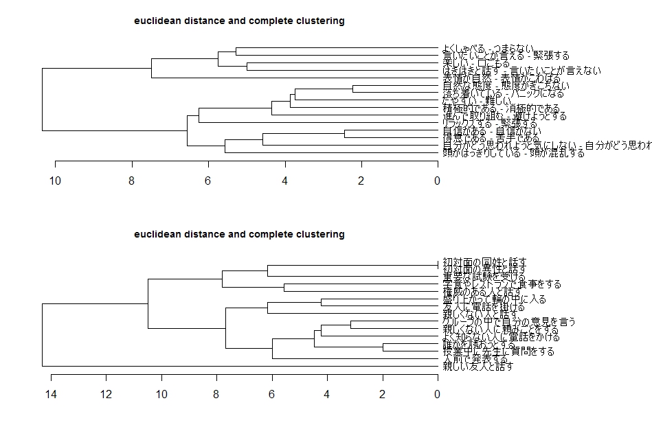
#クラスター分析を実施:clusterコマンド
#距離の計算方法を指定:dmethodオプション;"euclidean","maximum","manhattan",
#"canberra","binary","minkowski"が指定可能
#結合方法を指定:cmethodオプション;"ward","single","complete","average",
#"mcquitty","median","centroid"が指定可能
cluster(TestGrid, dmethod = "euclidean", cmethod = "complete")
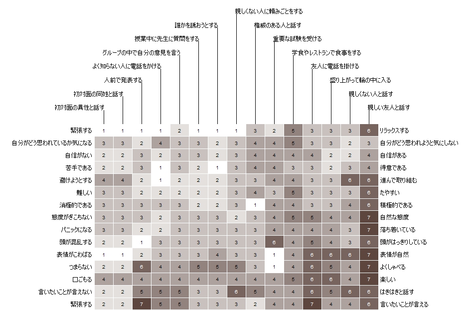
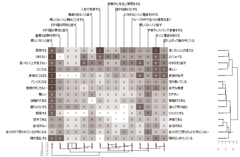
#bertinプロットの作成:bertinコマンド
#数値の表示:showvaluesオプション
#項目番号の表示:idオプション
bertin(TestGrid, color = c("white", "#5c463e"),
showvalues = TRUE, id = c(FALSE, FALSE))
#クラスタ付きのbertinプロットの作成:bertinClusterコマンド
bertinCluster(TestGrid, color = c("white", "#5c463e"),
showvalues = TRUE, id = c(FALSE, FALSE),
type = "rectangle", align = FALSE,
dmethod = c("euclidean", "euclidean"),
cmethod = c("complete", "complete"),
draw.axis = TRUE)
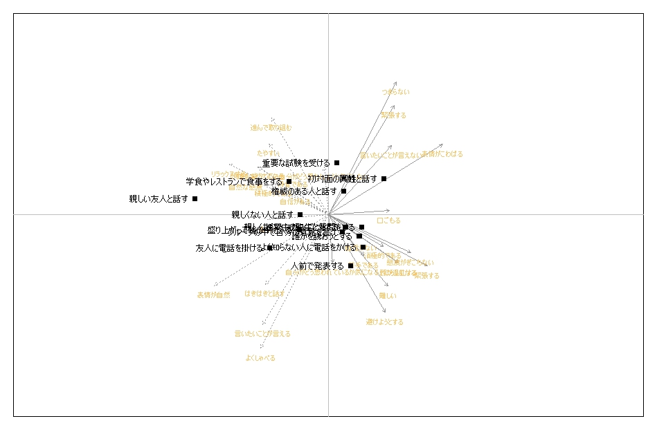
#biplotの作成:biplotSimpleコマンド
biplotSimple(TestGrid, c.label.col = "#f5c971")
出力例
・clusterコマンド
・bertinコマンド
・bertinClusterコマンド
・biplotSimpleコマンド
少しでも、あなたの解析が楽になりますように!!
けものフレンズ、奥が深いです。ぺぱぷらいぶ、気になります。