Rで解析：ggplot2で地図の描写や加工が楽々です「ggspatial」パッケージ

公開日 2022-07-10

「ggplot2」パッケージで地図の描写や加工が楽々なパッケージの紹介です。本パッケージはsfデータ以外にも緯度経度情報をデータフレームで与えることで、OpenStreetMapから地図を取得し描写と加工が可能です。なお、「ggplot2」パッケージのシステムを利用しているので、「ggplot2」パッケージのコマンドを組み合わせて使用することが可能です。

パッケージバージョンは1.1.6。実行コマンドはwindows 11のR version 4.1.3で確認しています。

＜おすすめのRに関する書籍です＞

RStudioではじめるRプログラミング入門 | ギャレット・グロ-ルマンド, 大橋真也, 長尾高弘

Amazonでギャレット・グロ-ルマンド, 大橋真也, 長尾高弘のRStudioではじめるRプログラミング入門。アマゾンならポイント還元本が多数。

www.amazon.co.jp

パッケージのインストール

下記コマンドを実行してください。

#パッケージのインストール
install.packages("ggspatial")

実行コマンド

詳細はコマンド、各パッケージのヘルプを確認してください。

#パッケージの読み込み
library("ggspatial")
###データを準備#####
#tidyverseパッケージがなければインストール
if(!require("tidyverse", quietly = TRUE)){
  install.packages("tidyverse");require("tidyverse")
}
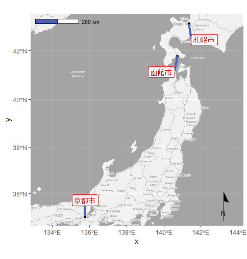
#札幌市役所,函館市役所,京都市役所の緯度経度
SKData <- tibble(x = c(141.3544, 140.7314, 135.7681),
                 y = c(43.0620, 41.7690, 35.0116),
                 city = c("札幌市", "函館市", "京都市"))
########
#プロット例
ggplot(SKData, aes(x, y)) +
  #OpenStreetMapの取得設定:annotation_map_tileコマンド
  #取得地図の形式を指定:typeオプション
  #"osm","opencycle","hotstyle","loviniahike","loviniacycle","hikebike"
  #"hillshade","osmgrayscale","stamenbw","stamenwatercolor","osmtransport"
  #"thunderforestoutdoors","cartodark","cartolight"
  #Map解像度の指定:zoominオプション;初期値:-2,解像度を上げるには-1/0を指定
  #透明度を指定:alphaオプション
  annotation_map_tile(type = "stamenbw", zoomin = 0, alpha = 0.3) +

  #取得地図にポイントを追加:geom_spatial_pointコマンド
  geom_spatial_point() +

  #取得地図にラベルを追加:geom_spatial_label_repelコマンド
  #ggrepel::geom_text_repelコマンドのオプションが使用可能
  #参考_https://www.karada-good.net/analyticsr/r-377/
  geom_spatial_label_repel(aes(label = city),
                           col = "red", segment.color = "#4b61ba",
                           segment.size = 1.5, box.padding = 1) +

  #スケールバーを追加:annotation_scaleコマンド
  #追加位置:locationオプション;"bl","br","tr","tl"
  #色を指定:bar_colsオプション
  annotation_scale(location = "tl",
                   bar_cols = c("#4b61ba", "white")) +

  #北向き矢印を追加:annotation_north_arrowコマンド
  #スタイルを指定:styleオプション;north_arrow_orienteering,
  #north_arrow_fancy_orienteering,north_arrow_minimal,
  #north_arrow_nautical;""は必要なし
  #北向きの基準:which_northオプション:"grid"/"true"
  annotation_north_arrow(style = north_arrow_minimal,
                         location = "br",
                         which_north = "true") +

  #width/heightを指定する:fixed_plot_aspectオプション
  fixed_plot_aspect(ratio = 1)
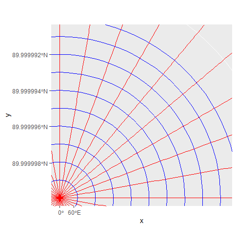
#経線緯線の描写:annotation_spatial_hline/annotation_spatial_vlineコマンド
ggplot(SKData, aes(x, y)) +
  coord_sf(crs = 3995) +
  #経線の描写:annotation_spatial_vlineコマンド
  annotation_spatial_vline(
    #線の描写間隔:interceptオプション
    intercept = seq(-180, 180, by = 10),
    crs = 4326, col = "red") +
  #緯線の描写:annotation_spatial_hlineコマンド
  annotation_spatial_hline(
    intercept = seq(89.999990, 90, by = 0.000001),
    crs = 4326, col = "blue")
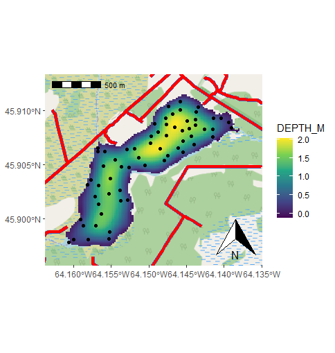
###その他参考#####
#パッケージ付属データを利用
load_longlake_data()
ggplot() +
  annotation_map_tile(zoomin = -1) +
  #sfデータを使用して道路情報をプロット
  annotation_spatial(longlake_roadsdf, size = 2, col = "#4b61ba") +
  annotation_spatial(longlake_roadsdf, size = 1.6, col = "red") +
  #sfデータを使用して湖情報をプロット
  layer_spatial(longlake_depth_raster) +
  #ggplot2::scale_fill_viridis_cコマンド
  scale_fill_viridis_c(na.value = NA) +
  layer_spatial(longlake_depthdf, aes(fill = DEPTH_M)) +
  annotation_scale(location = "tl") +
  annotation_north_arrow(location = "br", which_north = "true")