Rで解析:MATLABのいくつかのコマンドが使えます「matlab2r」パッケージ

Rの解析に役に立つ記事
スポンサーリンク

MATLABのいくつかのコマンドやMATLABのコマンドをRのコマンドに変換可能なパッケージの紹介です。

vector,matrix,array classの合計を計算、Aに含まれるがBに含まれないAのデータを表示、配列の変形、一様分布の配列を作成などの操作が可能なコマンドが収録されています。

パッケージバージョンは1.3.0。windows11のR version 4.2.2で確認しています。

スポンサーリンク

パッケージのインストール

下記コマンドを実行してください。

#パッケージのインストール
install.packages("matlab2r")

実行コマンド

詳細はコマンド、パッケージのヘルプを確認してください。

#パッケージの読み込み
library("matlab2r")

#条件がFALSEの時にエラーメッセージ:assertコマンド
#条件を設定:condオプション
#エラーメッセージを指定:msgオプション
#msgにC-styleフォーマットを含む場合:Aオプション
x <- FALSE
assert(cond = (x == TRUE),
       msg = "x is %s",
       A = class(x))

#&#25351;&#23450;&#12375;&#12383;&#25968;&#12398;&#21322;&#35282;&#31354;&#30333;&#12434;&#20316;&#25104;:blanks&#12467;&#12510;&#12531;&#12489;
blanks(n = 10)
#[1] "          "
#&#20363;&#12360;&#12400;
paste0("&#12363;&#12425;&#12384;&#12395;", blanks(n = 3), "&#12356;&#12356;&#12418;&#12398;")
#[1] "&#12363;&#12425;&#12384;&#12395;   &#12356;&#12356;&#12418;&#12398;"

#&#25991;&#23383;&#37197;&#21015;&#12434;&#20316;&#25104;:char&#12467;&#12510;&#12531;&#12489;
char(matrix(letters, 13))
#, , 1
#    [,1]
#[1,] "a" 
#[2,] "b" 
#[3,] "c" 
#[4,] "d" 
#[5,] "e" 
#[6,] "f" 
#[7,] "g" 
#[8,] "h" 
#[9,] "i" 
#[10,] "j" 
#[11,] "k" 
#[12,] "l" 
#[13,] "m" 

#, , 2
#   [,1]
#[1,] "n" 
#[2,] "o" 
#[3,] "p" 
#[4,] "q" 
#[5,] "r" 
#[6,] "s" 
#[7,] "t" 
#[8,] "u" 
#[9,] "v" 
#[10,] "w" 
#[11,] "x" 
#[12,] "y" 
#[13,] "z" 

#&#12505;&#12463;&#12488;&#12523;&#12434;&#20316;&#25104;:colon&#12467;&#12510;&#12531;&#12489;
#&#38283;&#22987;&#20516;:a&#12458;&#12503;&#12471;&#12519;&#12531;
#&#26368;&#32066;&#20516;:b&#12458;&#12503;&#12471;&#12519;&#12531;
colon(a = 8, b = 12)
[1]  8  9 10 11 12

#cat&#12467;&#12510;&#12531;&#12489;&#12398;&#12521;&#12483;&#12497;&#12540;:disp&#12467;&#12510;&#12531;&#12489;
TEST <- "&#12363;&#12425;&#12384;&#12395;&#12356;&#12356;&#12418;&#12398;"
disp(TEST)
&#12363;&#12425;&#12384;&#12395;&#12356;&#12356;&#12418;&#12398;
#&#20363;&#12360;&#12400;Test&#12434;&#23455;&#34892;&#12377;&#12427;&#12392;
TEST
#[1] "&#12363;&#12425;&#12384;&#12395;&#12356;&#12356;&#12418;&#12398;"

#&#20363;&#12360;&#12400;print&#12467;&#12510;&#12531;&#12489;
print(TEST)
#[1] "&#12363;&#12425;&#12384;&#12395;&#12356;&#12356;&#12418;&#12398;"

#&#20363;&#12360;&#12400;cat&#12467;&#12510;&#12531;&#12489;
cat(TEST)
#&#12363;&#12425;&#12384;&#12395;&#12356;&#12356;&#12418;&#12398;

#0&#12391;&#12399;&#12394;&#12356;&#25968;&#20516;&#12414;&#12383;&#12399;&#25351;&#23450;&#20516;&#12398;&#20301;&#32622;&#12434;&#21462;&#24471;:find&#12467;&#12510;&#12531;&#12489;
#&#25351;&#23450;&#20516;&#12399;&#12458;&#12502;&#12472;&#12455;&#12463;&#12488;&#12395;[==]&#12391;&#25351;&#23450;&#12377;&#12427;
#&#12487;&#12540;&#12479;&#12434;&#25351;&#23450;:x&#12458;&#12503;&#12471;&#12519;&#12531;
Test <- data.frame(data_1 = c(1, 0, 2, 0, 1),
                   data_2 = c(3, 1, 0, 0, 4))
find(x = Test)
#[1]  1  3  5  6  7 10
find(x = Test == 3)
#[1] 6

#&#23567;&#25968;&#28857;&#12398;&#20999;&#12426;&#25448;&#12390;:fix&#12467;&#12510;&#12531;&#12489;
fix(X = c(1.1, 0, 2.9, 3.5))
[1] 1 0 2 3
#trunc&#12467;&#12510;&#12531;&#12489;&#12392;&#21516;&#12376;
trunc(x = c(1.1, 0, 2.9, 3.5))
[1] 1 0 2 3

#&#12460;&#12531;&#12510;&#38306;&#25968;&#12398;&#33258;&#28982;&#23550;&#25968;&#12434;&#35336;&#31639;:gammaln&#12467;&#12510;&#12531;&#12489;
gammaln(A = c(1.1, 0, 2.9, 3.5))
[1] -0.04987244 Inf 0.60286961  1.20097360

#&#25991;&#23383;&#21015;&#12398;&#21322;&#35282;&#31354;&#30333;&#12434;1&#12391;&#36820;&#12377;:isspace&#12467;&#12510;&#12531;&#12489;
isspace(A = "&#12363;&#12425;&#12384;&#12395;&#12288;&#12356;&#12356; &#12418;&#12398; karada good")
[1] 0 0 0 0 0 0 0 1 0 0 1 0 0 0 0 0 0 1 0 0 0 0

#seq&#12467;&#12510;&#12531;&#12489;&#12398;&#12521;&#12483;&#12497;&#12540;:linspace&#12467;&#12510;&#12531;&#12489;
#&#38283;&#22987;&#20516;:x1&#12458;&#12503;&#12471;&#12519;&#12531;
#&#26368;&#32066;&#20516;:x2&#12458;&#12503;&#12471;&#12519;&#12531;
#&#38263;&#12373;:n&#12458;&#12503;&#12471;&#12519;&#12531;
linspace(x1 = -0.5, x2 = 5, n = 5L)
[1] -0.500  0.875  2.250  3.625  5.000
#&#20363;seq&#12467;&#12510;&#12531;&#12489;
seq(-0.5, 5, length.out = 5)

#Matlab&#12467;&#12510;&#12531;&#12489;&#12434;R&#12395;&#22793;&#25563;:matlab2r&#12467;&#12510;&#12531;&#12489;
#&#12497;&#12483;&#12465;&#12540;&#12472;&#21454;&#37682;&#12398;Matlab&#12467;&#12510;&#12531;&#12489;&#12434;&#35501;&#12415;&#36796;&#12416;
matlab_script <- system.file("extdata", "matlabDemo.m",
                             package = "matlab2r")
###matlabDemo.m&#12398;&#20869;&#23481;#####
read.table(matlab_script, sep = "\t")
#V1
#1                                                               function y = f(x)
#2  % This is a quick demonstration of MATLAB syntax. Its output is uninteresting.
#3                                                                         z = pi;
#4                                                                     if (z == 0)
#5                                                                         z = 10;
#6                                                                            else
#7                                                                       disp(OK);
#8                                                                             end
#9                                                                    for i = 1:10
#10                                                                    z2 = i - z;
#11                                                                            end
#12                                              y = z + x - (1 * 3 / 9) ^ 2 + z2;

#matlab2r&#12467;&#12510;&#12531;&#12489;
#&#22793;&#25563;&#26041;&#27861;&#12398;&#25351;&#23450;:output&#12458;&#12503;&#12471;&#12519;&#12531;
#&#22793;&#25563;&#24460;1&#34892;&#12372;&#12392;&#12467;&#12531;&#12477;&#12540;&#12523;&#20986;&#21147;;"asis",
#&#12467;&#12510;&#12531;&#12489;&#12392;&#12375;&#12390;&#12467;&#12531;&#12477;&#12540;&#12523;&#20986;&#21147;"clean"
#&#20803;&#12501;&#12449;&#12452;&#12523;&#12395;&#19978;&#26360;&#12365;"save"
#&#20803;&#12501;&#12449;&#12452;&#12523;&#12392;&#22793;&#25563;&#12467;&#12510;&#12531;&#12489;&#12434;&#12467;&#12531;&#12477;&#12540;&#12523;&#20986;&#21147;"diff"
matlab2r(matlab_script, output = "clean")
f <- function(x) {
  #  This is a quick demonstration of MATLAB syntax. Its output is uninteresting.
  z <- pi
  if ((z == 0)) {
    z <- 10
  } else {
    disp('OK')
  }
  for (i in 1:10) {
    z2 <- i - z
  }
  y <- z + x - (1 * 3 / 9) ^ 2 + z2
  return(y)
}
Warning message:
In matlab2r(matlab_script, output = "clean") :
Please pay special attention to parentheses. MATLAB uses them for both argument-passing and object-subsetting. The latter cases should be replaced by squared brackets.

#&#26368;&#22823;&#20516;&#12392;&#20301;&#32622;&#12434;&#21462;&#24471;:max&#12467;&#12510;&#12531;&#12489;
Test <- data.frame(data_1 = c(1, 0, 2, 0, 1),
                   data_2 = c(3, 1, 0, 0, 4))
#&#12487;&#12540;&#12479;&#12434;&#25351;&#23450;:X&#12458;&#12503;&#12471;&#12519;&#12531;
#&#20301;&#32622;&#21462;&#24471;:indices&#12458;&#12503;&#12471;&#12519;&#12531;;TRUE/FALSE
max(X = Test, indices = TRUE)
#$maxs
#data_1 data_2 
#2      4 
#$idx
#[1] 3 5

#&#26368;&#23569;&#20516;&#12392;&#20301;&#32622;&#12434;&#21462;&#24471;:min&#12467;&#12510;&#12531;&#12489;
Test <- matrix(c(1, 0, 2, 5, 1, 3))
#&#12487;&#12540;&#12479;&#12434;&#25351;&#23450;:X&#12458;&#12503;&#12471;&#12519;&#12531;
#&#20301;&#32622;&#21462;&#24471;:indices&#12458;&#12503;&#12471;&#12519;&#12531;;TRUE/FALSE
min(X = Test, indices = TRUE)
#$mins
#[1] 0
#$idx
#[1] 2

#&#25968;&#20516;&#12434;&#25991;&#23383;&#21015;&#12395;&#22793;&#25563;:num2str&#12467;&#12510;&#12531;&#12489;
#sprintf&#12467;&#12510;&#12531;&#12489;&#12398;fmt&#12458;&#12503;&#12471;&#12519;&#12531;&#12392;&#21516;&#12376;:format&#12458;&#12503;&#12471;&#12519;&#12531;
num2str(A = c(1.1, 0.0001, 2.9, 3.500),
        format = 5)
[1] "1.1"   "1e-04" "2.9"   "3.5" 

#&#35201;&#32032;&#12364;1&#12398;&#12510;&#12488;&#12522;&#12463;&#12473;&#12434;&#20316;&#25104;:ones&#12467;&#12510;&#12531;&#12489;
#&#34892;&#25968;&#12398;&#25351;&#23450;:n1&#12458;&#12503;&#12471;&#12519;&#12531;
#&#21015;&#25968;&#12398;&#25351;&#23450;:n2&#12458;&#12503;&#12471;&#12519;&#12531;
ones(n1 = 5, n2 = 2)
#     [,1] [,2]
#[1,]    1    1
#[2,]    1    1
#[3,]    1    1
#[4,]    1    1
#[5,]    1    1

#&#35201;&#32032;&#12364;0&#12398;&#12510;&#12488;&#12522;&#12463;&#12473;&#12434;&#20316;&#25104;:cell&#12467;&#12510;&#12531;&#12489;/zeros&#12467;&#12510;&#12531;&#12489;
cell(2, 3)
#     [,1] [,2] [,3]
#[1,]    0    0    0
#[2,]    0    0    0

zeros(2, 3)
#     [,1] [,2] [,3]
#[1,]    0    0    0
#[2,]    0    0    0

#&#19968;&#27096;&#20998;&#24067;&#12398;&#37197;&#21015;&#12434;&#20316;&#25104;:rand&#12467;&#12510;&#12531;&#12489;
#&#34892;&#25968;&#12398;&#25351;&#23450;:r&#12458;&#12503;&#12471;&#12519;&#12531;
#&#21015;&#25968;&#12398;&#25351;&#23450;:c&#12458;&#12503;&#12471;&#12519;&#12531;
rand(r = 3, c = 2)
#           [,1]       [,2]
#[1,] 0.81133714 0.45637136
#[2,] 0.21880174 0.48183421
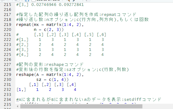
#[3,] 0.02746946 0.09272841

#&#25351;&#23450;&#12375;&#12383;&#37197;&#21015;&#12398;&#32368;&#12426;&#36820;&#12375;&#37197;&#21015;&#12434;&#20316;&#25104;:repmat&#12467;&#12510;&#12531;&#12489;
#&#32368;&#12426;&#36820;&#12375;&#25968;:n&#12458;&#12503;&#12471;&#12519;&#12531;;c(&#34892;&#26041;&#21521;,&#21015;&#26041;&#21521;),&#12418;&#12375;&#12367;&#12399;&#22238;&#25968;
repmat(mx = matrix(1:4, 2),
       n = c(2, 3))
#&#12288;&#12288;&#12288;[,1] [,2] [,3] [,4] [,5] [,6]
#[1,]    1    3    1    3    1    3
#[2,]    2    4    2    4    2    4
#[3,]    1    3    1    3    1    3
#[4,]    2    4    2    4    2    4

#&#37197;&#21015;&#12398;&#22793;&#24418;:reshape&#12467;&#12510;&#12531;&#12489;
#&#22793;&#24418;&#24460;&#12398;&#34892;&#25968;&#12434;&#25351;&#23450;:sz&#12458;&#12503;&#12471;&#12519;&#12531;;c(&#34892;&#25968;,&#21015;&#25968;)
reshape(A = matrix(1:4, 2),
        sz = c(1, 4))
     [,1] [,2] [,3] [,4]
[1,]    1    2    3    4

#A&#12395;&#21547;&#12414;&#12428;&#12427;&#12364;B&#12395;&#21547;&#12414;&#12428;&#12394;&#12356;A&#12398;&#12487;&#12540;&#12479;&#12434;&#34920;&#31034;:setdiff&#12467;&#12510;&#12531;&#12489;
setdiff(A = data.frame(data_1 = c(1, 0, 2, 9, 1),
                       data_2 = c(3, 1, 11, 0, 4)), 
        B = data.frame(data_1 = c(1, 0, 2, 0, 1),
                       data_2 = c(3, 1, 0, 8, 4)))
#&#12288;data_1 data_2
#3      2     11
#4      9      0

#&#12487;&#12540;&#12479;&#12398;&#20006;&#12403;&#26367;&#12360;:sortrows&#12467;&#12510;&#12531;&#12489;
#&#20006;&#12403;&#26367;&#12360;&#12398;&#21015;&#12434;&#25351;&#23450;:column&#12458;&#12503;&#12471;&#12519;&#12531;
sortrows(A = data.frame(data_1 = c(1, 0, 2, 9, 1),
                        data_2 = c(3, 1, 11, 0, 4)),
         column = 2)
  data_1 data_2
4      9      0
2      0      1
1      1      3
5      1      4
3      2     11

#vector,matrix,array class&#12398;&#21512;&#35336;&#12434;&#35336;&#31639;:sum_MATLAB&#12467;&#12510;&#12531;&#12489;
#&#35336;&#31639;&#26041;&#21521;&#12434;&#25351;&#23450;:dim&#12458;&#12503;&#12471;&#12519;&#12531;;&#21015;&#26041;&#21521;:1,&#34892;&#26041;&#21521;:2,&#20840;&#26041;&#21521;:"all"
sum_MATLAB(A = matrix(1:4, 2),
           dim = "all")
[1] 10

#&#12487;&#12540;&#12479;&#12398;&#25499;&#12369;&#31639;&#12364;&#31777;&#21336;:times&#12467;&#12510;&#12531;&#12489;
#data.frame class
Test <- data.frame(data_1 = c(1, 0, 2, 9, 1),
                   data_2 = c(3, 1, 11, 0, 4))
#&#25499;&#12369;&#12427;&#20516;&#12434;&#25351;&#23450;:b&#12458;&#12503;&#12471;&#12519;&#12531;
times(Test, b = 3)
#     data_1 data_2
#[1,]      3      9
#[2,]      0      3
#[3,]      6     33
#[4,]     27      0
#[5,]      3     12

#matrix class
Test <- matrix(1:4, 2)
times(Test, b = c(3, 0))
#     [,1] [,2]
#[1,]    3    9
#[2,]    0    0

少しでも、あなたの解析が楽になりますように!!

タイトルとURLをコピーしました