Rで解析：二次元データの色分け区分が楽々「biscale」パッケージ

二次元データの区分けが楽々できるパッケージの紹介です。区分け後のデータはパッケージ収録されている「bi_scale_fill」コマンドと凡例を作成する「bi_legend」コマンドを組み合わせて「ggplot2」パッケージでの利用が可能です。

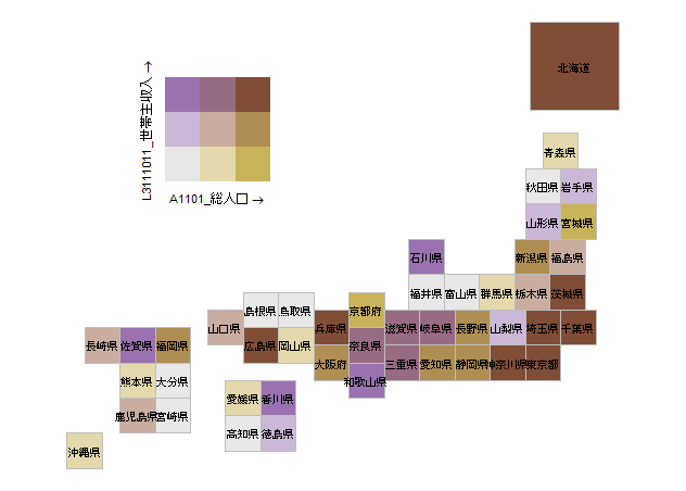
実行コマンドではe-Statで公開の2019年各都道府県の総人口（A1101）と世帯主収入（L3111011）を使用した区分けデータの作成例と「ggplot2」パッケージでの使用例を紹介します。

本パッケージは各コマンドの「dim」オプションを適切に設定することです。ミスがないように専用の変数を設定するのが良いかと思います。

パッケージバージョンは1.0.0。実行コマンドはwindows 11のR version 4.1.3で確認しています。

パッケージのインストール

下記コマンドを実行してください。

#&#12497;&#12483;&#12465;&#12540;&#12472;&#12398;&#12452;&#12531;&#12473;&#12488;&#12540;&#12523;
install.packages("biscale")

実行コマンド

詳細はコマンド、各パッケージのヘルプを確認してください。

#&#12497;&#12483;&#12465;&#12540;&#12472;&#12398;&#35501;&#12415;&#36796;&#12415;
library("biscale")

###&#12487;&#12540;&#12479;&#20363;&#12398;&#20316;&#25104;#####
#&#26085;&#26412;&#22320;&#22259;&#12487;&#12540;&#12479;&#12395;e-Stat&#12391;&#20844;&#38283;&#12398;2019&#24180;&#21508;&#37117;&#36947;&#24220;&#30476;&#12398;&#32207;&#20154;&#21475;&#65288;A1101&#65289;&#12392;
#&#19990;&#24111;&#20027;&#21454;&#20837;&#65288;L3111011&#65289;&#12487;&#12540;&#12479;&#12434;&#20184;&#19982;
#tidyverse&#12497;&#12483;&#12465;&#12540;&#12472;&#12364;&#12394;&#12369;&#12428;&#12400;&#12452;&#12531;&#12473;&#12488;&#12540;&#12523;
if(!require("tidyverse", quietly = TRUE)){
  install.packages("tidyverse");require("tidyverse")
}

JapanGrid <- tibble(
  #&#21508;&#37117;&#36947;&#24220;&#30476;&#12398;&#20301;&#32622;
  x = c(15.9, 15.5, 16, 16, 15.7, 15.7, 16, 15, 15, 14.7, 14.7, 15,
        15, 13.7, 14, 14, 12.7, 13, 13, 11.7, 11.7, 12, 12, 11, 11,
        10, 10, 10, 9, 9, 8, 8, 7, 7, 7.5, 7.5, 6.5, 6.5, 6, 4.5, 4.5,
        4.5, 3.5, 3.5, 3.5, 2.5, 2),
  y = c(12.9, 10.5, 9.5, 8.5, 7.5, 6.5, 5.5, 9.5, 8.5, 7.5, 6.5, 5.5,
        4.5, 6.5, 5.5, 4.5, 6.5, 5.5, 4.5, 7.5, 6.5, 5.5, 4.5, 5.5,
        4.5, 6, 5, 4, 5.5, 4.5, 6, 5, 6, 5, 3.5, 2.5, 3.5, 2.5, 5.5, 5, 4,
        3, 5, 4, 3, 5, 2),
  #width&#12392;height&#12399;&#12479;&#12452;&#12523;&#12398;&#22823;&#12365;&#12373;
  width = c(2.5, 1, 1, 1, 1, 1, 1, 1, 1, 1, 1, 1, 1, 1, 1, 1, 1, 1, 1, 1,
            1, 1, 1, 1, 1, 1, 1, 1, 1, 1, 1, 1, 1, 1, 1, 1, 1, 1, 1, 1, 1,
            1, 1, 1, 1, 1, 1),
  height = c(2.5, 1, 1, 1, 1, 1, 1, 1, 1, 1, 1, 1, 1, 1, 1, 1, 1, 1, 1, 1,
             1, 1, 1, 1, 1, 1, 1, 1, 1, 1, 1, 1, 1, 1, 1, 1, 1, 1, 1, 1, 1,
             1, 1, 1, 1, 1, 1),
  name = c("&#21271;&#28023;&#36947;", "&#38738;&#26862;&#30476;", "&#23721;&#25163;&#30476;", "&#23470;&#22478;&#30476;", "&#31119;&#23798;&#30476;",
           "&#33576;&#22478;&#30476;", "&#21315;&#33865;&#30476;", "&#31179;&#30000;&#30476;", "&#23665;&#24418;&#30476;", "&#26032;&#28511;&#30476;",
           "&#26627;&#26408;&#30476;", "&#22524;&#29577;&#30476;", "&#26481;&#20140;&#37117;", "&#32676;&#39340;&#30476;", "&#23665;&#26792;&#30476;",
           "&#31070;&#22856;&#24029;&#30476;", "&#23500;&#23665;&#30476;", "&#38263;&#37326;&#30476;", "&#38745;&#23713;&#30476;", "&#30707;&#24029;&#30476;",
           "&#31119;&#20117;&#30476;", "&#23696;&#38428;&#30476;", "&#24859;&#30693;&#30476;", "&#28363;&#36032;&#30476;", "&#19977;&#37325;&#30476;",
           "&#20140;&#37117;&#24220;", "&#22856;&#33391;&#30476;", "&#21644;&#27468;&#23665;&#30476;", "&#20853;&#24235;&#30476;", "&#22823;&#38442;&#24220;",
           "&#40165;&#21462;&#30476;", "&#23713;&#23665;&#30476;", "&#23798;&#26681;&#30476;", "&#24195;&#23798;&#30476;", "&#39321;&#24029;&#30476;", "&#24499;&#23798;&#30476;",
           "&#24859;&#23195;&#30476;", "&#39640;&#30693;&#30476;", "&#23665;&#21475;&#30476;", "&#31119;&#23713;&#30476;", "&#22823;&#20998;&#30476;", "&#23470;&#23822;&#30476;",
           "&#20304;&#36032;&#30476;", "&#29066;&#26412;&#30476;", "&#40575;&#20816;&#23798;&#30476;", "&#38263;&#23822;&#30476;", "&#27798;&#32260;&#30476;"),
  population = c(5250000, 1246000, 1227000, 2306000, 1846000, 2860000,
                 6259000, 966000, 1078000, 2223000, 1934000, 7350000,
                 13921000, 1942000, 811000, 9198000, 1044000, 2049000,
                 3644000, 1138000, 768000, 1987000, 7552000, 1414000,
                 1781000, 2583000, 1330000, 925000, 5466000, 8809000,
                 556000, 1890000, 674000, 2804000, 956000, 728000,
                 1339000, 698000, 1358000, 5104000, 1135000, 1073000,
                 815000, 1748000, 1602000, 1327000, 1453000),
  income = c(445412, 357657, 407047, 394064, 442343, 464558, 522793,
             388059, 432703, 442096, 437393, 604915, 541315, 369030,
             434731, 481065, 369259, 420433, 431561, 466789, 398272,
             448691, 426601, 473239, 484285, 354736, 453705, 445259,
             444813, 408470, 345036, 386071, 397061, 445291, 452776,
             403862, 399411, 379741, 418939, 429057, 381563, 343338,
             474686, 374987, 425488, 433126, 290871))
########

#&#65298;&#22793;&#25968;&#12398;&#22522;&#28310;&#12391;&#12487;&#12540;&#12479;&#12434;&#21306;&#20998;&#12377;&#12427;:bi_class&#12467;&#12510;&#12531;&#12489;
#&#20998;&#21106;&#22522;&#28310;:style&#12458;&#12503;&#12471;&#12519;&#12531;;"quantile","equal","fisher","jenks"
#&#20998;&#21106;&#25968;:dim&#12458;&#12503;&#12471;&#12519;&#12531;;2-4&#12398;&#31684;&#22258;
PlotData <- bi_class(.data = JapanGrid,
                     x = population, y = income,
                     style = "quantile", dim = 3)

#&#12300;ggplot2&#12301;&#12497;&#12483;&#12465;&#12540;&#12472;&#12391;&#21033;&#29992;&#12377;&#12427;&#20961;&#20363;&#12434;&#20316;&#25104;:bi_legend&#12467;&#12510;&#12531;&#12489;
#&#12459;&#12521;&#12540;&#12497;&#12524;&#12483;&#12488;&#12434;&#25351;&#23450;:pal&#12458;&#12503;&#12471;&#12519;&#12531;;"Bluegill","BlueGold","BlueOr",
#"BlueYl","Brown","Brown2","DkBlue","DkBlue2","DkCyan","DkCyan2",
#"DkViolet""DkViolet2","GrPink","GrPink2","PinkGrn","PurpleGrn","PurpleOr"
#&#12300;ggplot2&#12301;&#12497;&#12483;&#12465;&#12540;&#12472;&#12391;plot in plot&#12398;&#12383;&#12417;&#12395;ggplot2::ggplotGrob&#12467;&#12510;&#12531;&#12489;&#12434;&#21033;&#29992;
GG_legend <- ggplotGrob(bi_legend(pal = "Brown",
                                  dim = 3,
                                  xlab = "A1101_&#32207;&#20154;&#21475;",
                                  ylab = "L3111011_&#19990;&#24111;&#20027;&#21454;&#20837;",
                                  size = 8))

#&#12503;&#12525;&#12483;&#12488;
ggplot(data,
       aes(x = x, y = y, width = width, height = height)) +
  geom_tile(aes(fill = bi_class),
            color = "grey", show.legend = FALSE) +
  geom_text(aes(label = name), size = 2.6) +
  #&#22615;&#12426;&#12388;&#12406;&#12375;&#12434;&#36969;&#20999;&#12395;&#12362;&#12371;&#12394;&#12358;:bi_scale_fill&#12467;&#12510;&#12531;&#12489;
  bi_scale_fill(pal = "Brown", dim = 3) +
  coord_fixed(ratio = 1) +
  theme_void() +
  #&#20961;&#20363;&#12434;&#36861;&#21152;:ggplot2::annotation_custom&#12467;&#12510;&#12531;&#12489;
  annotation_custom(grob = GG_legend,
                    xmin = 3, xmax = 8,
                    ymin = 8, ymax = 14)

出力例

少しでも、あなたの解析が楽になりますように！！