オリジナルの地図データにグラフをプロット可能なパッケージの紹介です。地図データさえ用意できれば非常に有効なパッケージだと思います。参考までに日本地図データの作成例とプロット例を紹介します。
参考に気象庁から20220503の毎時の最高気温を取得して、各都道府県にヒートマップをプロットするコマンドも紹介します。
パッケージバージョンは0.2.0。実行コマンドはwindows 11のR version 4.1.3で確認しています。
日本地図データ例
お好みに合わせて、各都道府県の位置を調整してください。
#日本地図データの作成
JapanGrid <- data.frame(
row = c(1, 3, 4, 5, 6, 7, 8, 4, 5, 6,
7, 8, 9, 7, 8, 9, 7, 8, 9, 6,
7, 8, 9, 8, 9, 8, 9, 10, 8, 9,
8, 9, 8, 9, 11, 12, 11, 12, 9, 9,
10, 11, 9, 10, 11, 9, 12),
col = c(16, 16, 16, 16, 16, 16, 16, 15,
15, 15, 15, 15, 15, 14, 14, 14,
13, 13, 13, 12, 12, 12, 12, 11,
11, 10, 10, 10, 9, 9, 8, 8, 7, 7,
8, 8, 7, 7, 6, 4, 4, 4, 3, 3, 3, 2, 1),
code = c("北海道", "青森県", "岩手県", "宮城県", "福島県",
"茨城県", "千葉県", "秋田県", "山形県", "新潟県",
"栃木県", "埼玉県", "東京都", "群馬県", "山梨県",
"神奈川県", "富山県", "長野県", "静岡県", "石川県",
"福井県", "岐阜県", "愛知県", "滋賀県", "三重県",
"京都府", "奈良県", "和歌山県", "兵庫県", "大阪府",
"鳥取県", "岡山県", "島根県", "広島県", "香川県", "徳島県",
"愛媛県", "高知県", "山口県", "福岡県", "大分県", "宮崎県",
"佐賀県", "熊本県", "鹿児島県", "長崎県", "沖縄県"),
name = c("北海道", "青森県", "岩手県", "宮城県", "福島県",
"茨城県", "千葉県", "秋田県", "山形県", "新潟県",
"栃木県", "埼玉県", "東京都", "群馬県", "山梨県",
"神奈川県", "富山県", "長野県", "静岡県", "石川県",
"福井県", "岐阜県", "愛知県", "滋賀県", "三重県",
"京都府", "奈良県", "和歌山県", "兵庫県", "大阪府",
"鳥取県", "岡山県", "島根県", "広島県", "香川県", "徳島県",
"愛媛県", "高知県", "山口県", "福岡県", "大分県", "宮崎県",
"佐賀県", "熊本県", "鹿児島県", "長崎県", "沖縄県"))
#作業フォルダに日本地図データを保存
write.csv(JapanGrid, "JapanGrid.csv", row.names = FALSE)
########パッケージのインストール
下記コマンドを実行してください。
#パッケージのインストール
install.packages("geofacet")
実行コマンド
詳細はコマンド、パッケージのヘルプを確認してください。体裁はggplot2のコマンドで調整可能です。
#パッケージの読み込み
library("geofacet")
library("ggplot2")
library("tcltk")
#先に作成した地図データを読み込む
JapanGrid <- read.csv(paste0(as.character(tkgetOpenFile(title = "ファイルを選択",
filetypes = '{"ファイル" {".*"}}',
initialfile = c("*.*")))))
########
###データ例を作成#####
TestJPN <- data.frame(Year = factor(rep(2015:2017, times = nrow(JapanGrid))),
Temp = sample(10:20, size = nrow(JapanGrid)*3, replace = TRUE),
Name = rep(JapanGrid[, 4], each = 3))
########
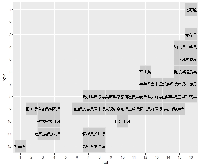
#地図データを表示:grid_previewコマンド
grid_preview(JapanGrid)
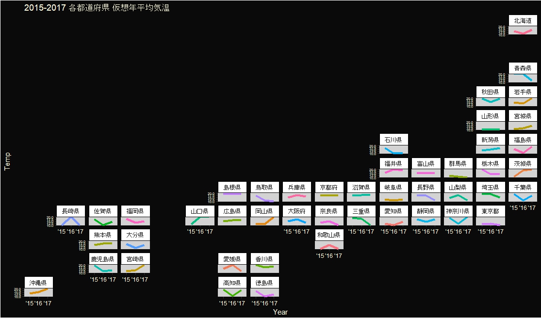
#地図データを利用してデータをプロット:facet_geoコマンド
#データの分割方法:facetsオプション;facet_wrapコマンドと同じ
#地図データを指定:gridオプション
ggplot(TestJPN, aes(x = Year, y = Temp, group = Name, col = Name)) +
geom_line(show.legend = FALSE, size = 1.5) +
facet_geo(facets = ~ Name, grid = JapanGrid) +
scale_x_discrete(labels = function(x) paste0("'", substr(x, 3, 4))) +
scale_y_continuous(labels = function(x) format(x, 2)) +
labs(title = "2015-2017 各都道府県 仮想年平均気温") +
theme(title = element_text(colour = "#ffffe0"),
axis.title = element_text(colour = "#ffffe0"),
axis.text = element_text(colour = "#ffffe0"),
strip.text.x = element_text(size = 8),
strip.background = element_rect(colour = "black", fill = "white"),
axis.text.y = element_text(size = 5),
panel.grid = element_blank(),
panel.background = element_rect(fill = "lightgray"),
plot.background = element_rect(fill = "#0a0a0a"))
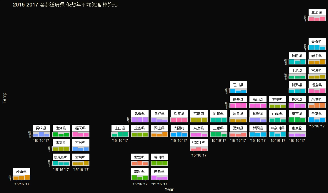
#参考:棒グラフで表示
ggplot(TestJPN, aes(x = Year, y = Temp, group = Name, fill = Name)) +
geom_col(show.legend = FALSE) +
facet_geo(facets = ~ Name, grid = JapanGrid) +
scale_x_discrete(labels = function(x) paste0("'", substr(x, 3, 4))) +
scale_y_continuous(labels = function(x) format(x, 2)) +
labs(title = "2015-2017 各都道府県 仮想年平均気温 棒グラフ") +
theme(title = element_text(colour = "#ffffe0"),
axis.title = element_text(colour = "#ffffe0"),
axis.text = element_text(colour = "#ffffe0"),
strip.text.x = element_text(size = 8),
strip.background = element_rect(colour = "black", fill = "white"),
axis.text.y = element_text(size = 5),
panel.grid = element_blank(),
panel.background = element_rect(fill = "lightgray"),
plot.background = element_rect(fill = "#0a0a0a"))出力例
各グラフはクリックで大きく見ることができます。
・grid_previewコマンド
・地図データを利用してデータをプロット:facet_geoコマンド
・参考:棒グラフで表示
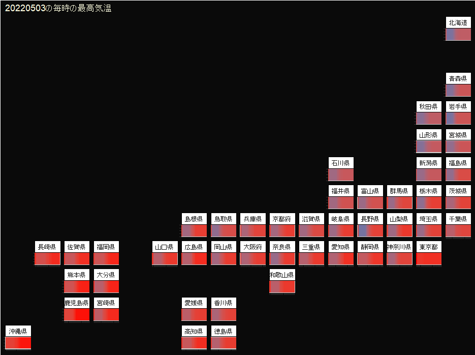
最高気温を気象庁から取得してプロット
気象庁から20220503の毎時の最高気温を取得した例です。データを変えると最高気温以外もプロット可能です。
データを取得
###データ例を作成#####
#「tidyverse」パッケージを読み込み
if(!require("tidyverse", quietly = TRUE)){
install.packages("tidyverse");require("tidyverse")
}
#都道府県を準備
JpanName <- c("北海道", "青森県", "岩手県", "宮城県", "福島県", "茨城県", "千葉県",
"秋田県", "山形県", "新潟県", "栃木県", "埼玉県", "東京都", "群馬県",
"山梨県", "神奈川県", "富山県", "長野県", "静岡県", "石川県", "福井県",
"岐阜県", "愛知県", "滋賀県", "三重県", "京都府", "奈良県", "和歌山県",
"兵庫県", "大阪府", "鳥取県", "岡山県", "島根県", "広島県", "香川県",
"徳島県", "愛媛県", "高知県", "山口県", "福岡県", "大分県", "宮崎県",
"佐賀県", "熊本県", "鹿児島県", "長崎県", "沖縄県")
#時間文字列を作成
Hour <- paste0(formatC(0:23, width = 2, flag = "0"), "00")
#データ保管用変数
NewMaxTemp <- data.frame()
for(i in seq(Hour)){
###気象庁から20220503の毎時の最高気温を取得#####
#参考:https://www.data.jma.go.jp/obd/stats/data/mdrr/docs/csv_dl_readme.html
MaxTemp <- read.csv(paste0("https://www.data.jma.go.jp/obd/stats/data/mdrr/tem_rct/alltable/mxtemsadext00_20220503", Hour[i], ".csv"),
header = T, fileEncoding = "cp932")
#最高気温処理
GetMaxTemp <- NULL
for(n in 1:47){
#都道府県を抽出
GetNameData <- MaxTemp[which(MaxTemp[, 2] %in% grep(JpanName[n], MaxTemp[, 2], value = TRUE)),]
#最高気温を降順で並び替え
GetNameData <- GetNameData[order(GetNameData[, 10], decreasing = TRUE),]
#最高気温を取得
GetMaxTemp <- c(GetMaxTemp, GetNameData[1, 10])
}
HourTemp <- cbind(Hour[i], JpanName, GetMaxTemp)
NewMaxTemp <- rbind(NewMaxTemp, HourTemp)
}
#列名を付与
colnames(NewMaxTemp) <- c("Hour", "Name", "MaxTemp")
#最高気温を数値化
NewMaxTemp[, 3] <- type.convert(NewMaxTemp[, 3], as.is = TRUE)
#Hourをfactor化
NewMaxTemp %>%
mutate(Hour = factor(Hour)) -> NewMaxTemp
########プロット
#パッケージの読み込み
library("geofacet")
#先に作成した地図データを読み込む
JapanGrid <- read.csv(paste0(as.character(tkgetOpenFile(title = "ファイルを選択",
filetypes = '{"ファイル" {".*"}}',
initialfile = c("*.*")))))
#プロット
ggplot(NewMaxTemp, aes(x = Hour, y = 1, group = Name, fill = MaxTemp)) +
geom_tile(show.legend = FALSE, size = 1.5) +
facet_geo(facets = ~ Name, grid = JapanGrid) +
scale_fill_gradient(low = "#6f74a4", high = "red") +
labs(title = "20220503の毎時の最高気温") +
theme(title = element_text(colour = "#ffffe0"),
axis.title = element_text(colour = "#ffffe0"),
axis.text = element_text(colour = "#ffffe0"),
strip.text.x = element_text(size = 8),
strip.background = element_rect(colour = "black", fill = "white"),
axis.text.y = element_blank(),
axis.text.x = element_blank(),
axis.title.x = element_blank(),
axis.title.y = element_blank(),
panel.grid = element_blank(),
panel.background = element_rect(fill = "lightgray"),
plot.background = element_rect(fill = "#0a0a0a"))出力例
グラフはクリックで大きく見ることができます。
少しでも、あなたの解析が楽になりますように!!