Rで解析：t検定からANOVAまで幅広く対応と検出力分析など「ggpower」パッケージの紹介

医療統計や臨床試験の計画では、研究デザインやサンプルサイズの計算に多くの時間を割くことがあります。特に、t検定やANOVA、回帰分析などの検出力やサンプルサイズの計算です。本パッケージは、t検定、ANOVA、回帰分析、χ二乗検定、比例検定、相関分析、非パラメトリック検定など、多くの研究デザインに対応した検出力分析とサンプルサイズの計算が可能です。

パッケージバージョンは0.1.2。Windows 11 x64 (build 26200)のR version 4.6.1で確認しています。

＜おすすめのRに関する書籍です＞

R／RStudioでやさしく学ぶプログラミングとデータ分析【ダウンロード特典付き！】 | 掌田津耶乃

掌田津耶乃作品ほか、お急ぎ便対象商品は当日お届けも可能。またR／RStudioでやさしく学ぶプログラミングとデータ分析【ダウンロード特典付き！】もアマゾン配送商品なら通常配送無料。

www.amazon.co.jp

パッケージのインストール

下記コマンドを実行してください。

# パッケージのインストール
install.packages("ggpower")
# パッケージの読み込み
library("ggpower")

コマンド例

詳細はコメント、パッケージのヘルプを確認してください。

一標本t検定の検出力を計算：power_t_one_sampleコマンド

# 効果サイズが0.5の場合の1標本検定の検出力計算
power_t_one_sample(d = 0.5, n = 40, alpha = 0.05)

実行結果：

[1] 0.8693981

対応のあるt検定の検出力を計算：power_t_pairedコマンド

# 対応のあるt検定の検出力計算
power_t_paired(d = 0.5, n = 20)

実行結果：

[1] 0.5645044

分布関数を使った計算スクリプトを評価：ggpower_calculatorコマンド

# z値を計算するためのggpower calculatorの使用例
ggpower_calculator("x <- 2^3\nx + zinv(.975)")

実行結果：

[1] 9.959964

＜おすすめのRに関する書籍です＞

基礎から学ぶ統計学 | 中原 治

Amazonで中原 治の基礎から学ぶ統計学。アマゾンならポイント還元本が多数。中原 治作品ほか、お急ぎ便対象商品は当日お届けも可能。また基礎から学ぶ統計学もアマゾン配送商品なら通常配送無料。

www.amazon.co.jp

統計的有意性の分析結果に基づく実験デザインの最適化：power_computeコマンド

# t検定の検出力計算（事前分布あり）
power_compute("t_one_sample", "a_priori", d = 0.625, alpha = 0.05,
  power = 0.95, tails = "one")

実行結果：

ggpower result
Test: t test: Means - difference from constant (one sample case)
Analysis: a_priori

Input parameters
  tails: greater
  effect_size_d: 0.625
  alpha: 0.05
  total_sample_size: 30
  target_power: 0.95


Output parameters
  noncentrality_parameter: 3.423266
  critical_t: 1.699127
  df: 29
  actual_power: 0.9551444


Notes
…(以下略)

対応している統計検定の一覧を取得：ggpower_testsコマンド

サポートされている統計的検定手法を確認できます。

# 検定手法を表示 
ggpower_tests()
ggpower_tests(module = "biomarker")

実行結果：

# 検定手法を表示 
ggpower_tests()$ id
 [1] "t_one_sample"                   "t_paired"                       "t_two_sample"                  
 [4] "t_point_biserial"               "t_linear_regression"            "t_linear_regression_two_groups"
 [7] "t_generic"                      "f_anova_one_way"                "f_anova_special"               
[10] "f_mreg_omnibus"                 "f_mreg_increase"                "f_variance_two"                
[13] "chisq_variance_one"             "chisq_gof"                      "chisq_contingency"             
[16] "exact_binomial"                 "exact_one_proportion"           "exact_sign"                    
[19] "exact_fisher"                   "exact_mcnemar"                  "exact_correlation"             
[22] "exact_mreg_random"              "z_corr_independent"             "z_corr_dependent_common"       
[25] "z_corr_dependent_no_common"     "z_logistic"                     "z_poisson"                     
[28] "z_tetrachoric"                  "wilcoxon_signed"                "wilcoxon_mann_whitney"         
[31] "roc_auc_one"                    "roc_auc_two"                    "diagnostic_acc"                
[34] "survival_logrank"               "cox_regression"                 "discovery_fdr"                 
[37] "ttest_biomarker"                "rct_superiority_continuous"     "rct_superiority_binary"        
[40] "rct_noninferiority_continuous"  "rct_noninferiority_binary"      "rct_equivalence_continuous"    
[43] "rct_equivalence_proportion"     "simon_two_stage"                "cluster_rct"                   
[46] "multi_arm_superiority"          "count_endpoint_poisson"         "survival_pmu"    

一標本t検定の検出力曲線をプロット：ggpower_t_one_sampleコマンド

# 効果サイズが0.5の場合の1標本検定の検出力曲線のプロット
ggpower_t_one_sample(d = 0.5, alpha = 0.05, n_range = seq(20, 100, by = 5))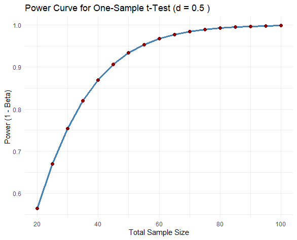

＜おすすめのRに関する書籍です＞

サラっとできる!フリー統計ソフトEZR(Easy R)でカンタン統計解析 | 神田 善伸

Amazonで神田 善伸のサラっとできる!フリー統計ソフトEZR(Easy R)でカンタン統計解析

www.amazon.co.jp

任意の検定の検出力曲線をプロット：plot_power_curveコマンド

実行すると、指定された分析方法や検定手法に基づく検出力曲線が得られます。固定パラメータに対して使用される検出力分析モードとGoogleで検索するとanalysisオプションの意味がよくわかります。

# survival_pmuのプロット
plot_power_curve("survival_pmu", n_values = c(200, 300, 400), analysis = "post_hoc")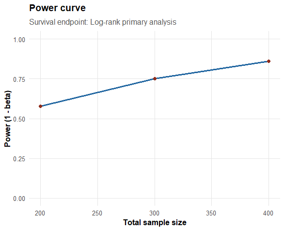

帰無仮説と対立仮説の分布を可視化：plot_distributionコマンド

# t検定を計算する
result <- power_compute("t_one_sample", "post_hoc", d = 0.5, n = 40)

# 計算結果の分布をプロットする
plot_distribution(result)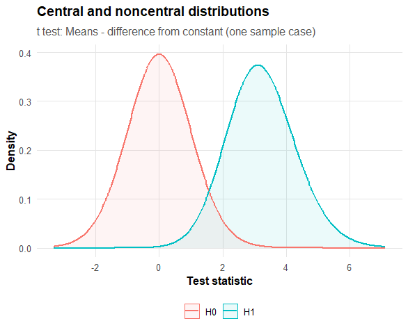

＜おすすめのRに関する書籍です＞

R／RStudioでやさしく学ぶプログラミングとデータ分析【ダウンロード特典付き！】 | 掌田津耶乃

掌田津耶乃作品ほか、お急ぎ便対象商品は当日お届けも可能。またR／RStudioでやさしく学ぶプログラミングとデータ分析【ダウンロード特典付き！】もアマゾン配送商品なら通常配送無料。

www.amazon.co.jp

この記事が誰かの役に立ちますように。