「 1つの変数:連続変数 」、「2つの変数: 連続変数、離散変数の組み合わせ」による「ggplot2」パッケージでのプロット例です。各データ例のコマンドも紹介していますので、プロットに対するデータ形式の参考にしてください。
なお、「ggplot2」パッケージ を利用するために「tidyverse」パッケージを使用します。
パッケージバージョンは1.3.1。実行コマンドはwindows 11のR version 4.1.2で確認しています。
パッケージのインストール
下記、コマンドを実行してください。
#パッケージのインストール
install.packages("tidyverse")
実行コマンド
・「tidyverse」パッケージの読み込みとデータ例の作成
#パッケージの読み込み
library("tidyverse")
###データ例の作成#####
set.seed(1234)
n <- 300
TestData <- tibble(Group = sample(paste0("Group", 1:4), n,
replace = TRUE),
X_num_Data = sample(c(1:50), n, replace = TRUE),
Y_num_Data = sample(c(51:100), n, replace = TRUE),
Chr_Data = sample(c("か", "ら", "だ", "に",
"い", "い", "も", "の"),
n, replace = TRUE),
Fct_Data = factor(sample(c("か", "ら", "だ", "に",
"い", "い", "も", "の"),
n, replace = TRUE)))
#確認
TestData
# A tibble: 300 x 5
Group X_num_Data Y_num_Data Chr_Data Fct_Data
<chr> <int> <int> <chr> <fct>
1 Group4 31 83 だ い
2 Group4 33 95 か に
3 Group2 45 74 ら い
4 Group2 10 99 い い
5 Group1 22 90 の だ
6 Group4 13 65 い に
7 Group3 27 76 い ら
8 Group1 40 66 だ ら
9 Group1 18 92 い も
10 Group2 23 84 の も
#######・1つの変数:連続変数で作成できるプロット
#基本となるggplot2のデータ作成
One_Cotinuous <- ggplot(TestData, aes(x = X_num_Data,
color = Group,
fill = Group))
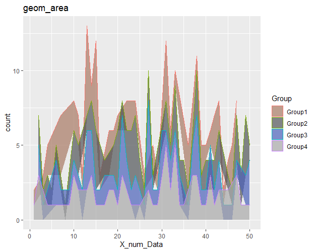
#geom_areaコマンド
#集計方法を設定:statオプション;"bin","count","density"などがあります
One_Cotinuous +
geom_area(stat = "count", alpha = 0.7) +
scale_fill_manual(values = c("#a87963", "#505457",
"#4b61ba", "#A9A9A9")) +
labs(title = "geom_area")
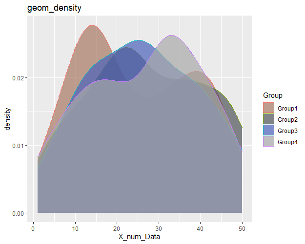
#geom_densityコマンド
One_Cotinuous +
geom_density(alpha = 0.7) +
scale_fill_manual(values = c("#a87963", "#505457",
"#4b61ba", "#A9A9A9")) +
labs(title = "geom_density")
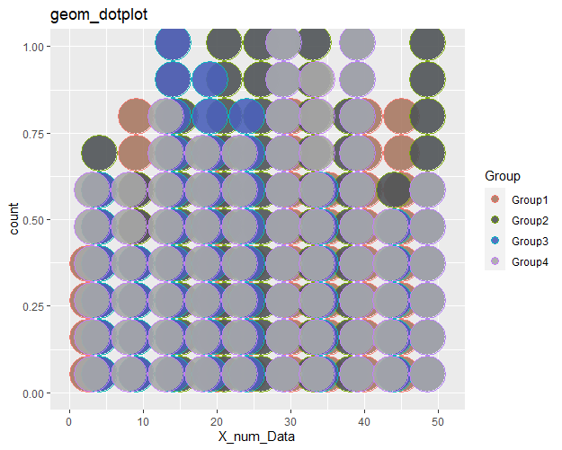
#geom_dotplotコマンド
#ビンの表示手法:methodオプション;"dotdensity","histodot"
One_Cotinuous +
geom_dotplot(method = "dotdensity", binwidth = 5, alpha = 0.9) +
scale_fill_manual(values = c("#a87963", "#505457",
"#4b61ba", "#A9A9A9")) +
labs(title = "geom_dotplot")
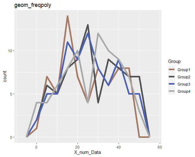
#geom_freqpolyコマンド
One_Cotinuous +
geom_freqpoly(binwidth = 5, size = 2) +
scale_color_manual(values = c("#a87963", "#505457",
"#4b61ba", "#A9A9A9")) +
labs(title = "geom_freqpoly")
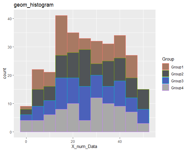
#geom_histogramコマンド
One_Cotinuous +
geom_histogram(binwidth = 5) +
scale_fill_manual(values = c("#a87963", "#505457",
"#4b61ba", "#A9A9A9")) +
labs(title = "geom_histogram")
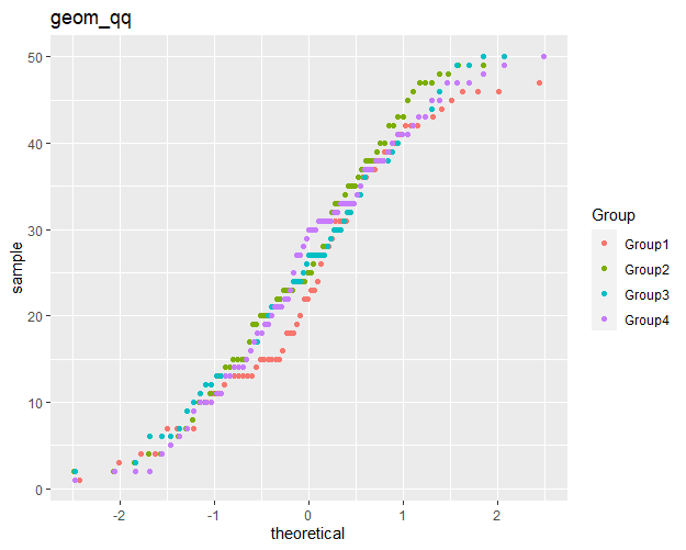
#geom_qqコマンド
ggplot(TestData) +
geom_qq(aes(sample = X_num_Data, colour = Group)) +
scale_fill_manual(values = c("#a87963", "#505457",
"#4b61ba", "#A9A9A9")) +
labs(title = "geom_qq")
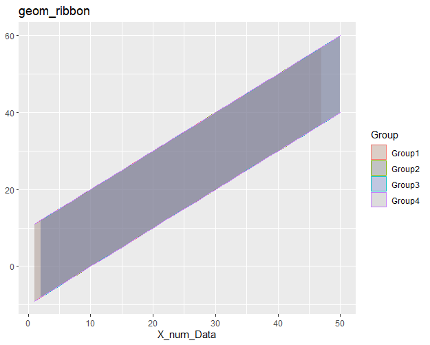
#geom_ribbonコマンド
One_Cotinuous +
geom_ribbon(aes(ymin = X_num_Data - 10, ymax = X_num_Data + 10),
alpha = 0.3) +
scale_fill_manual(values = c("#a87963", "#505457",
"#4b61ba", "#A9A9A9")) +
labs(title = "geom_ribbon")【出力例】
・2つの変数:x、y共に連続変数 で作成できるプロット
#基本となるggplot2のデータ作成
Two_Cotinuous <- ggplot(TestData, aes(x = X_num_Data,
y = Y_num_Data,
color = Group,
fill = Group))
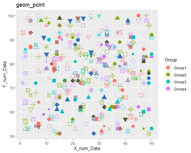
#geom_pointコマンド
#シンボルを指定:shapeオプション;0:25まで指定可能
#例では全種類プロット
Two_Cotinuous +
geom_point(alpha = 1, size = 4, shape = rep(0:25, length = 300)) +
scale_fill_manual(values = c("#a87963", "#505457",
"#4b61ba", "#A9A9A9")) +
labs(title = "geom_point")
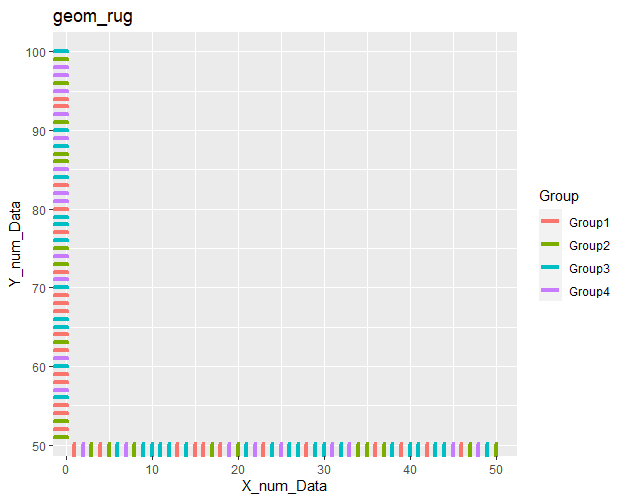
#geom_rugコマンド
Two_Cotinuous +
geom_rug(size = 1.5) +
scale_fill_manual(values = c("#a87963", "#505457",
"#4b61ba", "#A9A9A9")) +
labs(title = "geom_rug")
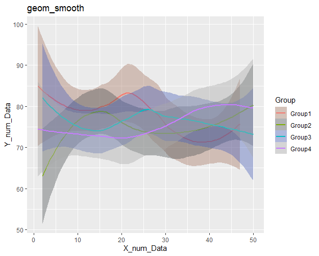
#geom_smoothコマンド
Two_Cotinuous +
geom_smooth() +
scale_fill_manual(values = c("#a87963", "#505457",
"#4b61ba", "#A9A9A9")) +
labs(title = "geom_smooth")
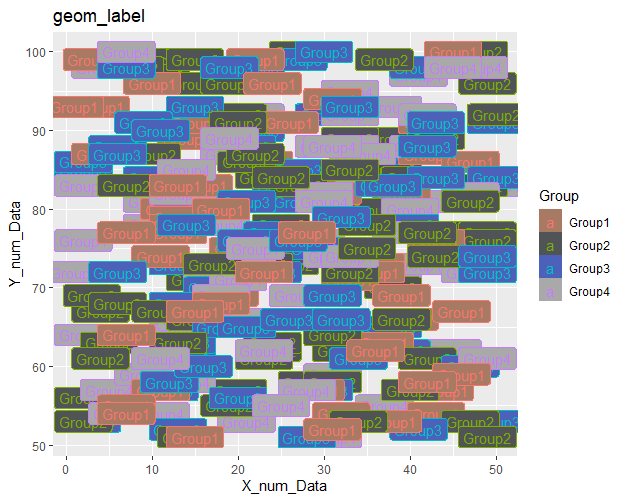
#geom_labelコマンド
Two_Cotinuous +
geom_label(aes(label = Group)) +
scale_fill_manual(values = c("#a87963", "#505457",
"#4b61ba", "#A9A9A9")) +
labs(title = "geom_label")
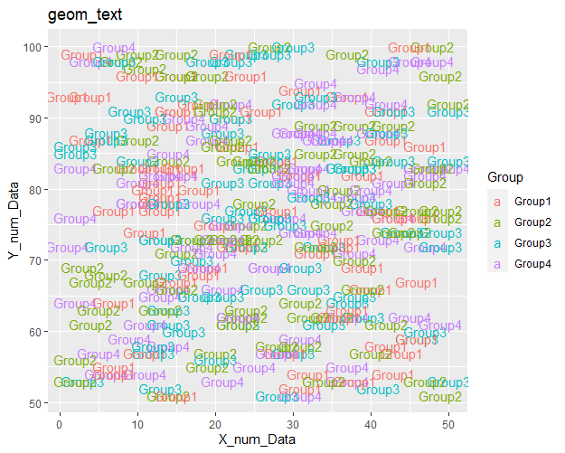
#geom_textコマンド
Two_Cotinuous +
geom_text(aes(label = Group)) +
scale_fill_manual(values = c("#a87963", "#505457",
"#4b61ba", "#A9A9A9")) +
labs(title = "geom_text")【出力例】
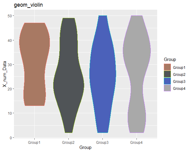
・2つの変数:離散変数、連続変数の組み合わせで作成できるプロット
#基本となるggplot2のデータ作成
#プロットが見やすくなるようデータを100まで使用
Discrete_Cotinuous <- ggplot(TestData[1:100,],
aes(x = Group, y = X_num_Data,
color = Group, fill = Group))
#geom_violinコマンド
Discrete_Cotinuous +
geom_violin() +
scale_fill_manual(values = c("#a87963", "#505457",
"#4b61ba", "#A9A9A9")) +
labs(title = "geom_violin")
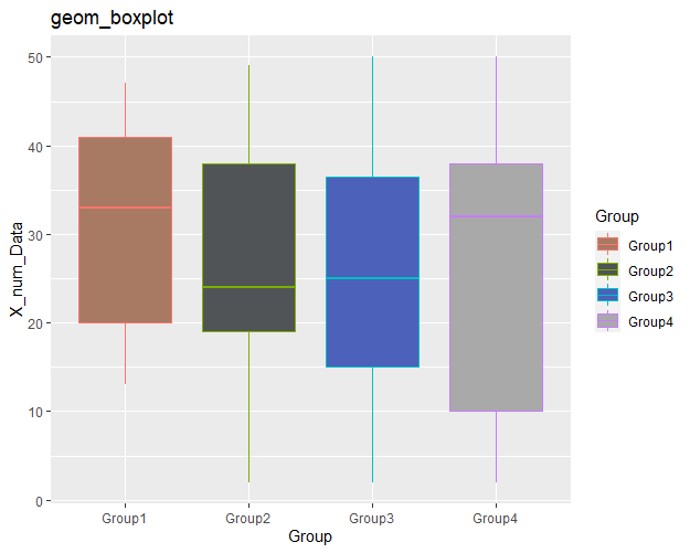
#geom_boxplotコマンド
Discrete_Cotinuous +
geom_boxplot() +
scale_fill_manual(values = c("#a87963", "#505457",
"#4b61ba", "#A9A9A9")) +
labs(title = "geom_boxplot")
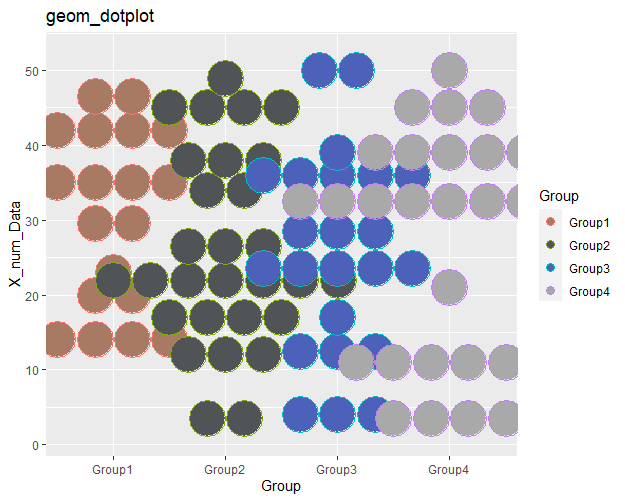
#geom_dotplotコマンド
#ドットの表示方法:stackdirオプション;"up","down","center","centerwhole"
Discrete_Cotinuous +
geom_dotplot(binaxis = "y", stackdir = "center", binwidth = 5) +
scale_fill_manual(values = c("#a87963", "#505457",
"#4b61ba", "#A9A9A9")) +
labs(title = "geom_dotplot")
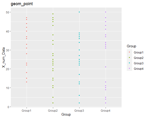
#geom_pointコマンド
Discrete_Cotinuous +
geom_point(size = 1) +
scale_fill_manual(values = c("#a87963", "#505457",
"#4b61ba", "#A9A9A9")) +
labs(title = "geom_point")【出力例】
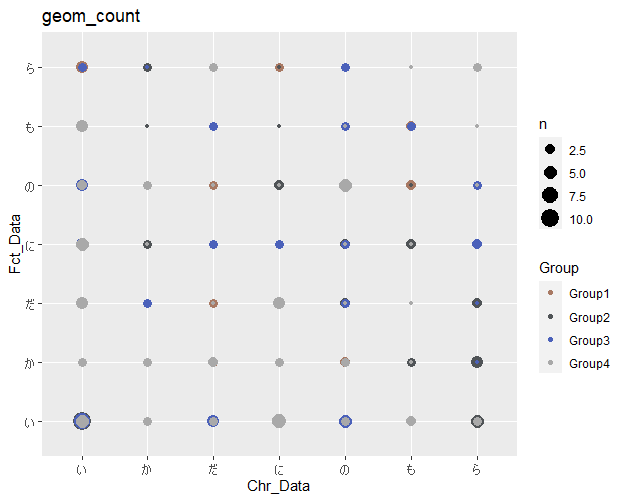
・2つの変数:x、y共に離散変数の組み合わせで作成できるプロット
#基本となるggplot2のデータ作成
Two_Discrete <- ggplot(TestData, aes(x = Chr_Data,
y = Fct_Data,
color = Group,
fill = Group))
#geom_countコマンド
Two_Discrete +
geom_count() +
scale_color_manual(values = c("#a87963", "#505457",
"#4b61ba", "#A9A9A9")) +
labs(title = "geom_count")
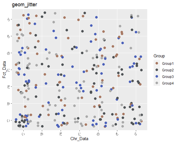
#geom_jitterコマンド
Two_Discrete +
geom_jitter(size = 3) +
scale_color_manual(values = c("#a87963", "#505457",
"#4b61ba", "#A9A9A9")) +
labs(title = "geom_jitter")【出力例】
少しでも、あなたの解析が楽になりますように!!