Rで解析：カテゴリ数が違っても棒グラフの幅をそろえる「ggwidth」パッケージの紹介

データ分析や可視化において、ggplot2は非常に便利なツールです。しかし、棒グラフでは、プロットごとに見た目の幅が異なってしまうことがあります。この問題を解決するパッケージの紹介です。

パッケージバージョンは0.1.1。Windows 11 x64 (build 26200)のR version 4.6.1で確認しています。

＜おすすめのRに関する書籍です＞

RStudioではじめるRプログラミング入門 | ギャレット・グロ-ルマンド, 大橋真也, 長尾高弘

Amazonでギャレット・グロ-ルマンド, 大橋真也, 長尾高弘のRStudioではじめるRプログラミング入門。アマゾンならポイント還元本が多数。

www.amazon.co.jp

パッケージのインストール

下記コマンドを実行してください。

# パッケージのインストール
install.packages("ggwidth")
# パッケージの読み込み
library("ggwidth")
# コマンド例実行で必要なパッケージを読み込み
library("ggplot2")
library("dplyr")
library("patchwork")

コマンド例

詳細はコメント、パッケージのヘルプを確認してください。

全ての図に適用する幅の倍率をまとめて設定：set_equiwidthコマンド

# 等幅の設定
set_equiwidth(1)
set_equiwidth(0.75)
set_equiwidth(1.33)

カテゴリ数やパネルサイズが異なっても見た目の幅を統一：get_widthコマンド

# パネルの幅・高さを指定したテーマを設定
set_theme(
  theme_grey() +
    theme(panel.widths  = rep(unit(75, "mm"), 2)) +
    theme(panel.heights = rep(unit(50, "mm"), 2))
)
# 幅のスケーリング係数を初期化
set_equiwidth(1)

# カテゴリ数3の縦向き棒グラフ
p1 <- mpg |>
  ggplot(aes(x = drv)) +
  geom_bar(
    width = get_width(n = 3),
    colour = "black",
    fill = "grey",
  )

# カテゴリ数7の縦向き棒グラフ
p2 <- diamonds |>
  ggplot(aes(x = color)) +
  geom_bar(
    width = get_width(n = 7),
    colour = "black",
    fill = "grey",
  )

# カテゴリ数7の横向き棒グラフ
p3 <- diamonds |>
  ggplot(aes(y = color)) +
  geom_bar(
    width = get_width(n = 7, orientation = "y"),
    colour = "black",
    fill = "grey",
  )

# ドッジされた棒グラフ（カテゴリ数3、ドッジ数4）
p4 <- mpg |>
  ggplot(aes(x = drv, group = factor(cyl))) +
  geom_bar(
    position = position_dodge(preserve = "single"),
    width = get_width(n = 3, n_dodge = 4),
    colour = "black",
    fill = "grey",
  )

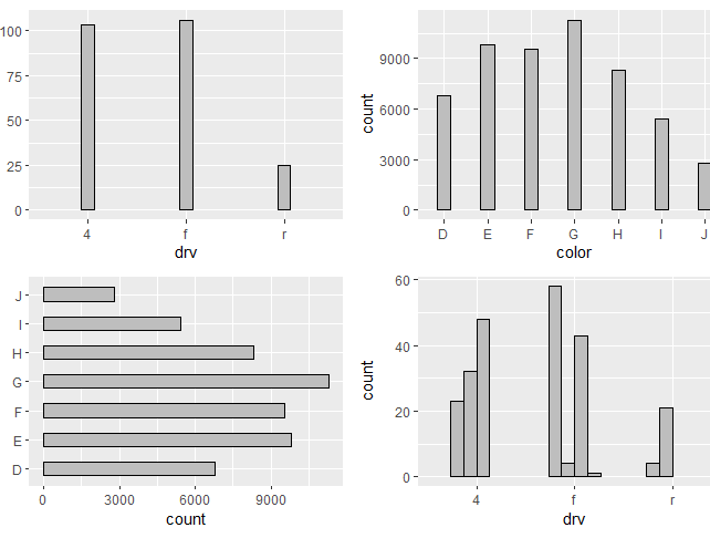
# 4つのプロットを並べて表示し、幅の見た目がそろっていることを確認
p1 + p2 + p3 + p4

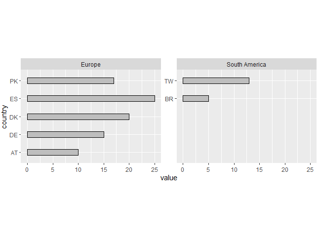
# ファセット分割用のサンプルデータを作成
d <- tibble::tibble(
  continent = c("Europe", "Europe", "Europe", "Europe", "Europe",
                "South America", "South America"),
  country   = c("AT", "DE", "DK", "ES", "PK", "TW", "BR"),
  value     = c(10L, 15L, 20L, 25L, 17L, 13L, 5L)
)

# 各大陸の中でカテゴリ数が最大のものを取得
max_n <- d |>
  count(continent) |>
  pull(n) |>
  max()

# ファセットごとにカテゴリ数が異なっても、幅の見た目をそろえて表示
d |>
  mutate(country = forcats::fct_rev(country)) |>
  ggplot(aes(y = country, x = value)) +
  geom_col(
    width = get_width(n = max_n, orientation = "y"),
    colour = "black",
    fill = "grey",
  ) +
  facet_wrap(~continent, scales = "free_y") +
  scale_y_discrete(continuous.limits = c(1, max_n)) +
  coord_cartesian(reverse = "y", clip = "off")

# パネル幅を指定する場合
mpg |>
  ggplot(aes(x = drv)) +
  geom_bar(
    width = get_width(n = 3, panel_widths = unit(160, "mm")),
    colour = "black",
    fill = "grey",
  ) +
  theme(panel.widths = unit(160, "mm"))

・4つのプロットを並べて表示し、幅の見た目がそろっていることを確認

・ファセットごとにカテゴリ数が異なっても、幅の見た目をそろえて表示

・パネル幅を指定する場合

＜おすすめのRに関する書籍です＞

R言語ではじめるプログラミングとデータ分析 | 馬場 真哉

Amazonで馬場 真哉のR言語ではじめるプログラミングとデータ分析。アマゾンならポイント還元本が多数。馬場 真哉作品ほか、お急ぎ便対象商品は当日お届けも可能。

www.amazon.co.jp

この記事が誰かの役に立ちますように。