 からだにいいもの
 Rで解析:変数の型から相関手法を自動選択する「smartcor」パッケージの紹介
変数の性質に合った相関係数を選ぶことは、解析結果を誤って解釈しないために重要です。しかし、連続値・カウント・二値・順序・カテゴリカルといった型を一つずつ見極め、変数のペアごとに手法を割り当てる作業には手間がかかります。「smartcor」パッケージは、変数の統計的タイプの判定から相関手法の選択と計算までを一括しておこなえるパッケージです。ベクトルの型を判定するコマンドや、型の組み合わせに応じた手法で相関係数を算出するコマンドが収録されています。PearsonやSpearman、Kendallのタウのほか、四分相関、多分相関、CramerのVなど14種類の手法に対応し、信頼区間とp値の算出が可能です。なお、手法を選んだ理由を含む結果を整然データ形式へ変換したり、相関行列をヒートマップでプロット可能です。
パッケージバージョンは1.0.1。Windows 11 x64 (build 26200)のR version 4.6.1で確認しています。
パッケージのインストール
下記コマンドを実行してください。
# パッケージのインストール
install.packages("smartcor")

# パッケージの読み込み
library("smartcor")コマンド例
詳細はコメント、パッケージのヘルプを確認してください。
本パッケージで判定可能な値は、continuous(連続値)、count(非負の整数値)、binary(二値:YES/NOなど)、ordinal(順序尺度)、categorical(カテゴリカル)の5種類です。
解説に使用するサンプルデータの作成
以降のコマンド例では、架空の和菓子店24店舗の来店調査データを使用します。5種類の統計的タイプがすべて含まれるように作成しています。
# 和菓子店24店舗の来店調査を想定したオリジナルデータを作成
wagashi <- data.frame(

  # 店名
  mise = c("甘露堂", "初雪庵", "花見月", "白露堂", "松風庵", "雪華堂",
           "千歳屋", "三日月堂", "藤乃屋", "山桜堂", "竹葉庵", "磯乃香",
           "柚子乃木", "紅葉屋", "清流庵", "木漏日堂", "蓮池屋", "稲穂庵",
           "霜柱堂", "春告堂", "夕凪庵", "峰の雪", "綿雲堂", "星月夜"),

  # 平均滞在時間(分) continuous(連続値)
  taizai = c(18.4, 25.1, 31.7, 14.2, 28.9, 35.6, 21.3, 16.8,
             33.2, 27.4, 12.6, 38.1, 22.7, 19.5, 29.3, 24.8,
             36.9, 15.4, 30.2, 26.1, 41.5, 17.9, 23.6, 32.8),

  # 一日平均来店者数(人)
  raiten = c(119, 89, 140, 103, 147, 159, 65, 110,
             173, 126, 93, 260, 143, 118, 148, 131,
             236, 45, 212, 178, 207, 67, 160, 222),

  # 味の満足度(5段階評価) ordinal(順序尺度)
  aji = c(3, 4, 5, 2, 4, 5, 3, 3, 5, 4, 2, 5,
          4, 3, 4, 4, 5, 2, 4, 4, 5, 3, 3, 5),

  # 雰囲気の満足度(5段階評価)
  funiki = c(3, 3, 5, 2, 4, 5, 4, 2, 4, 4, 2, 5,
             3, 3, 5, 4, 5, 3, 4, 3, 5, 2, 4, 4),

  # 実演販売の有無(binary)
  jitsuen = c("なし", "あり", "あり", "なし", "あり", "あり",
              "なし", "なし", "あり", "あり", "なし", "あり",
              "あり", "なし", "あり", "あり", "あり", "なし",
              "あり", "あり", "あり", "なし", "なし", "あり"),
  # 所在する地方(カテゴリカル)
  chihou = c(rep("北海道", 6), rep("東北", 6),
             rep("関東", 6), rep("関西", 6)),

  # 文字列を因子に変換しない
  stringsAsFactors = FALSE
)
変数の統計的タイプを自動判別:detect_typeコマンド
| オプション | 意味 | 初期値 |
|---|---|---|
| x | 数値・因子・文字列または論理ベクトルを指定 | なし |
| ordinal_threshold | 順序尺度と判定する固有値数の上限を整数で指定 | 10 |
| detect_count | 非負の整数値をカウント型と判定するか否かを論理値で指定 | TRUE |
| verbose | 判定理由の出力有無を論理値で指定 | FALSE |
ベクトルのクラスと欠損値を除いた固有値の数から、5種類の統計的タイプのいずれかを文字列として返します。順序付き因子は常にordinal、固有値が2つの文字列や論理値はbinary、固有値がordinal_thresholdを超える非負の整数値はcountと判定されます。verboseにTRUEを指定すると、判定理由がメッセージとして出力されます。
# 平均滞在時間の統計的タイプを判定
detect_type(wagashi$taizai)
[1] "continuous"

# 味の満足度の統計的タイプを判定
detect_type(wagashi$aji)
ordinal(順序尺度)

# 順序尺度とみなす固有値数の上限を3に下げて判定
# 固有値が4つのため順序尺度から外れ、非負の整数値としてカウント型になる
detect_type(wagashi$aji, ordinal_threshold = 3)
[1] "count"

# カウント型の判定を無効にして一日平均来店者数を判定
detect_type(wagashi$raiten, detect_count = FALSE)
[1] "continuous"

# データフレームの全列に対してまとめて判定
vapply(wagashi, detect_type, character(1))
   mise        taizai        raiten           aji        funiki       jitsuen        chihou
"categorical"  "continuous"       "count"     "ordinal"     "ordinal"      "binary" "categorical"
型の組み合わせで使える手法を一覧:available_methodsコマンド
| オプション | 意味 | 初期値 |
|---|---|---|
| type_x | “continuous”、”count”、”binary”、”ordinal”、”categorical”のいずれかを指定 | なし |
| type_y | “continuous”、”count”、”binary”、”ordinal”、”categorical”のいずれかを指定 | なし |
2つの統計的タイプの組み合わせに対して算出できる手法を、コード名のmethod列と説明のlabel列を持つtibbleとして返します。
# 順序尺度どうしの組み合わせで利用できる手法を確認
available_methods("ordinal", "ordinal")
# A tibble: 4 × 2
  method     label
  <chr>      <chr>
1 polychoric Polychoric Correlation
2 kendall    Kendall's Tau-b
3 spearman   Spearman Rank Correlation
4 gamma      Goodman-Kruskal's Gamma

# 連続値と二値の組み合わせで利用できる手法を確認
available_methods("continuous", "binary")
  method         label
  <chr>          <chr>
1 pearson        Pearson Correlation
2 point_biserial Point-Biserial Correlation (= Pearson)

# 判定結果をそのまま渡して利用できる手法を確認
available_methods(detect_type(wagashi$taizai), detect_type(wagashi$chihou))
# A tibble: 1 × 2
 method    label
 <chr>     <chr>
1 cramers_v Cramer's V
2変数に最適な相関手法を選択して計算:smart_corコマンド
| オプション | 意味 | 初期値 |
|---|---|---|
| x | 同じ長さの数値、因子、文字列または論理ベクトルを指定 | なし |
| y | 同じ長さの数値、因子、文字列または論理ベクトルを指定 | なし |
| x_type | 自動判定を上書きする”continuous”、”count”、”binary”、”ordinal”、”categorical”のいずれかを指定 | NULL |
| y_type | 自動判定を上書きする”continuous”、”count”、”binary”、”ordinal”、”categorical”のいずれかを指定 | NULL |
| method | 手法を固定する”pearson”、”spearman”、”kendall”、”phi”、”tetrachoric”、”yules_q”、”polychoric”、”polyserial”、”cramers_v”、”theils_u”、”tschuprows_t”、”gamma”、”rank_biserial”、”point_biserial”のいずれかを指定 | NULL |
| assume_latent_normal | 潜在正規性の扱いを”auto”、論理値またはNULLで指定 | “auto” |
| ordinal_threshold | detect_typeコマンドに渡す整数値を指定 | 10 |
| ignore_na | 欠損値を含む行を除去するか否かを論理値で指定 | TRUE |
| conf_level | 信頼区間の水準を0から1の数値で指定 | 0.95 |
| bootstrap | ブートストラップ推論の実行を”auto”、TRUEまたはFALSEで指定 | “auto” |
| n_boot | ブートストラップの反復回数を整数で指定 | 500 |
| n_perm | TheilのUのp値を求める置換回数を整数で指定 | 500 |
| seed | ブートストラップと置換抽出の乱数シードを整数で指定 | NULL |
| verbose | 判定と選択の過程を示すメッセージの出力有無を論理値で指定 | TRUE |
2変数の統計的タイプを判定し、その組み合わせに応じた手法で相関係数、統計量、p値、信頼区間を算出します。assume_latent_normalに”auto”を指定した場合はtest_bivariate_normalityコマンドによる尤度比カイ二乗検定の結果で手法を決定し、TRUEでは多分相関や四分相関などの潜在変数を仮定する手法を、FALSEではKendallのタウやSpearmanなどの順位相関系を選択します。NULLを指定すると対話的に選択になります。


# 平均滞在時間と一日平均来店者数の相関を自動選択で算出
# 連続値とカウントの組み合わせのためPearsonの積率相関が選択される
smart_cor(wagashi$taizai, wagashi$raiten)
── Variable types ──

ℹ Detected as continuous (numeric with 24 unique values).
wagashi$taizai: "continuous"
ℹ Detected as count (non-negative integer with 24 unique values).
wagashi$raiten: "count"

── Method selection ──

✔ Selected: Pearson Correlation (count treated as continuous)

── Smart Correlation ───────────────────────────────────────────────────────────────────────────────
Estimate: 0.8190
Method: Pearson Correlation (count treated as continuous)
Variables: wagashi$taizai ("continuous") × wagashi$raiten ("count")
N: 24
p-value: < 0.001
Test: t-test on r (cor.test)
H0: rho = 0
Small p-values (e.g., p < 0.05) indicate evidence against H0.
95% CI: [0.6206, 0.9188]
Source: Fisher z (cor.test)

One variable is continuous and the other is a count. Counts are treated as numeric continuous
variables; Pearson correlation selected (matches base R cor()).

ℹ Alternatives: "spearman" and "kendall" (pass `method = "..."` to use)


# 平均滞在時間と実演販売の有無の相関を算出
# 連続値と二値の組み合わせのためPoint-biserial correlation;点双列相関(点二列相関)が選択される
smart_cor(wagashi$taizai, wagashi$jitsuen, verbose = FALSE)
── Smart Correlation ───────────────────────────────────────────────────────────────────────────────
Estimate: -0.8117
Method: Point-Biserial Correlation (= Pearson)
Variables: wagashi$taizai ("continuous") × wagashi$jitsuen ("binary")
N: 24
p-value: < 0.001
Test: t-test on r (cor.test)
H0: rho_pb = 0
Small p-values (e.g., p < 0.05) indicate evidence against H0.
95% CI: [-0.9154, -0.6071]
Source: Fisher z (cor.test); = Pearson

One variable is continuous and the other is binary. Point-biserial correlation is mathematically
identical to Pearson when the binary variable is coded 0/1.

# 味と雰囲気の満足度の相関を潜在正規性を仮定せずに算出
# 順序尺度どうしのためKendallのタウが選択される
smart_cor(wagashi$aji, wagashi$funiki,
          assume_latent_normal = FALSE, verbose = FALSE)
── Smart Correlation ───────────────────────────────────────────────────────────────────────────────
Estimate: 0.7079
Method: Kendall's Tau-b
Variables: wagashi$aji ("ordinal") × wagashi$funiki ("ordinal")
N: 24
p-value: < 0.001
Test: asymptotic normal (cor.test, exact = FALSE)
H0: tau = 0
Small p-values (e.g., p < 0.05) indicate evidence against H0.
95% CI: [0.5322, 0.8251]
Source: Fieller, Hartley, and Pearson (1957)

Both variables are ordinal. Kendall's tau selected (no latent normality assumption; stable bias
                                                    across distributions).

ℹ Alternatives: "polychoric", "spearman", and "gamma" (pass `method = "..."` to use)

# 手法をSpearmanの順位相関に固定して算出
smart_cor(wagashi$taizai, wagashi$raiten,
          method = "spearman", verbose = FALSE)
── Smart Correlation ───────────────────────────────────────────────────────────────────────────────
Estimate: 0.8322
Method: Spearman Rank Correlation
Variables: wagashi$taizai ("continuous") × wagashi$raiten ("count")
N: 24
p-value: < 0.001
Test: t approximation (cor.test, exact = FALSE)
H0: rho_S = 0
Small p-values (e.g., p < 0.05) indicate evidence against H0.
95% CI: [0.6037, 0.9343]
Source: Bonett and Wright (2000)

Method selected by user: spearman

# 味の満足度と地方の関連をブートストラップ信頼区間つきで算出
# 順序尺度とカテゴリカルの組み合わせのためCramerのVが選択される
smart_cor(wagashi$aji, wagashi$chihou,
          bootstrap = TRUE, n_boot = 1000, seed = 1234, verbose = FALSE)
── Smart Correlation ───────────────────────────────────────────────────────────────────────────────
Estimate: 0.2073
Method: Cramer's V (ordinal ordering ignored)
Variables: wagashi$aji ("ordinal") × wagashi$chihou ("categorical")
N: 24
p-value: 0.9604
Test: Pearson chi-square test of independence
H0: variables are independent
Small p-values indicate evidence that the variables are not independent.
95% CI (bootstrap): [0.2478, 0.5464]
Source: Percentile bootstrap

One variable is ordinal and the other is categorical. Cramer's V selected (ordinal ordering
                                                                           ignored).
適用できる手法をまとめて比較:compare_methodsコマンド
| オプション | 意味 | 初期値 |
|---|---|---|
| x | 同じ長さの数値、因子、文字列または論理ベクトルを指定 | なし |
| y | 同じ長さの数値、因子、文字列または論理ベクトルを指定 | なし |
| x_type | 自動判定を上書きする”continuous”などの文字列を指定 | NULL |
| y_type | 自動判定を上書きする”continuous”などの文字列を指定 | NULL |
| assume_latent_normal | 推奨フラグの決定方法を”auto”または論理値で指定 | “auto” |
| ordinal_threshold | detect_typeコマンドに渡す整数値を指定 | 10 |
| ignore_na | 欠損値を含む行を除去するか否かを論理値で指定 | TRUE |
| conf_level | 表の各区間における信頼水準を0から1の数値で指定 | 0.95 |
| bootstrap | ブートストラップの対象を”auto”、TRUEまたはFALSEで指定 | “auto” |
| n_boot | 手法あたりのブートストラップ反復回数を整数で指定 | 500 |
| n_perm | TheilのUのp値を求める置換回数を整数で指定 | 500 |
| seed | ブートストラップと置換抽出の乱数シードを整数で指定 | NULL |
| verbose | 情報メッセージの出力有無を論理値で指定 | TRUE |

2変数の組み合わせに適用できる手法をすべて算出し、推定値、統計量、p値、信頼区間を一覧にしたsmartcor_comparisonクラスのオブジェクトを返します。既定で選択される手法にはrecommended列にTRUEが立つため、手法間で結果がどの程度異なるかを確認できます。まぁ、いいのかな?よくわからない。
# 味と雰囲気の満足度に適用できる手法をまとめて比較
# 順序尺度どうしのため多分相関、Kendall、Spearman、ガンマが算出される
compare_methods(wagashi$aji, wagashi$funiki,
                assume_latent_normal = FALSE, bootstrap = FALSE,
                verbose = FALSE)
── Method Comparison ───────────────────────────────────────────────────────────────────────────────
Variables: wagashi$aji ("ordinal") × wagashi$funiki ("ordinal")
N: 24

Polychoric Correlation
r = 0.8631 p < 0.001 95% CI [0.6201, 0.9550]
Kendall's Tau-b ← recommended
r = 0.7079 p < 0.001 95% CI [0.5322, 0.8251]
Spearman Rank Correlation
r = 0.7865 p < 0.001 95% CI [0.5174, 0.9140]
Goodman-Kruskal's Gamma
r = 0.8817 p < 0.001 95% CI [0.6783, 0.9596]

# 信頼水準を99%に変更し、全手法をブートストラップで比較
compare_methods(wagashi$taizai, wagashi$raiten,
                conf_level = 0.99, bootstrap = TRUE,
                n_boot = 1000, seed = 1234, verbose = FALSE)
── Method Comparison ───────────────────────────────────────────────────────────────────────────────
Variables: wagashi$taizai ("continuous") × wagashi$raiten ("count")
N: 24

Pearson Correlation ← recommended
r = 0.8190 p < 0.001 99% CI [0.6765, 0.9132]
Spearman Rank Correlation
r = 0.8322 p < 0.001 99% CI [0.5755, 0.9456]
Kendall's Tau-b
r = 0.6522 p < 0.001 99% CI [0.4448, 0.8315]
潜在的な二変量正規性を検定:test_bivariate_normalityコマンド
| オプション | 意味 | 初期値 |
|---|---|---|
| x | 順序尺度もしくは二値のベクトル、または集計表を指定 | なし |
| y | 順序尺度もしくは二値のベクトルを指定し、集計表を渡す場合はNULLとする | NULL |
| alpha | 検定の有意水準を数値で指定 | 0.05 |
| max_levels | 集計表作成時のカテゴリ数の上限を整数で指定 | 10L |
集計表に対して閾値モデルを最尤推定し、潜在的な二変量正規分布への当てはまりを尤度比カイ二乗検定で確認します。返り値は統計量、自由度、p値、多分相関の推定値、各変数の閾値などを含むsmartcor_normtestクラスのオブジェクトです。max_levelsを超える固有値を持つ数値ベクトルは、指定数の分位群に区分されてから集計表が作成されます。
# 味と雰囲気の満足度が潜在的な二変量正規分布に従うかを検定
test_bivariate_normality(wagashi$aji, wagashi$funiki)
── Bivariate Normality Test (LR Chi-Square) ──

Table dimensions: 4 x 4
N = 24
Polychoric rho: 0.8628
LR chi-square: 2.4331 (df = 8, p = 0.9648)
Conclusion: no evidence against bivariate normality at alpha = 0.05. Polychoric correlation is
appropriate.

# 有意水準を1%に変更して検定
test_bivariate_normality(wagashi$aji, wagashi$funiki, alpha = 0.01)
── Bivariate Normality Test (LR Chi-Square) ──

Table dimensions: 4 x 4
N = 24
Polychoric rho: 0.8628
LR chi-square: 2.4331 (df = 8, p = 0.9648)
Conclusion: no evidence against bivariate normality at alpha = 0.01. Polychoric correlation is
appropriate.

# 集計表を作成
hyou <- table(wagashi$aji, wagashi$funiki)

# 作成済みの集計表を直接渡して検定
test_bivariate_normality(hyou)
── Bivariate Normality Test (LR Chi-Square) ──

Table dimensions: 4 x 4
N = 24
Polychoric rho: 0.8628
LR chi-square: 2.4331 (df = 8, p = 0.9648)
Conclusion: no evidence against bivariate normality at alpha = 0.05. Polychoric correlation is
appropriate.

# 一日平均来店者数を4分位群に区分してから順序尺度との検定をおこなう
test_bivariate_normality(wagashi$raiten, wagashi$aji, max_levels = 4L)
── Bivariate Normality Test (LR Chi-Square) ──

Table dimensions: 4 x 4
N = 24
Polychoric rho: 0.8121
LR chi-square: 2.5733 (df = 8, p = 0.9582)
Conclusion: no evidence against bivariate normality at alpha = 0.05. Polychoric correlation is
appropriate.
データフレームから相関行列を作成:smart_cormatコマンド
| オプション | 意味 | 初期値 |
|---|---|---|
| data | データフレームまたはtibbleを指定 | なし |
| cols | 対象とする列名の文字列ベクトルを指定 | NULL |
| types | 列名と統計的タイプを対応づけた名前付きリストを指定 | NULL |
| assume_latent_normal | 潜在正規性の扱いを”auto”、論理値またはNULLで指定 | “auto” |
| ordinal_threshold | detect_typeコマンドに渡す整数値を指定 | 10 |
| ignore_na | 欠損値をペアごとに処理するか否かを論理値で指定 | TRUE |
| conf_level | 各ペアに渡す信頼水準を0から1の数値で指定 | 0.95 |
| bootstrap | ブートストラップの対象を”auto”、TRUEまたはFALSEで指定 | “auto” |
| n_boot | ペアあたりのブートストラップ反復回数を整数で指定 | 500 |
| n_perm | TheilのUのp値を求める置換回数を整数で指定 | 500 |
| seed | ブートストラップと置換抽出の乱数シードを整数で指定 | NULL |
| verbose | 進捗情報の出力有無を論理値で指定 | TRUE |

データフレームの各列についてすべてのペアの相関を算出し、相関行列、使用した手法の行列、判定された型、ペアごとの詳細を持つsmartcormatクラスのオブジェクトを返します。表示すると、変数の型、相関行列、手法の2文字略号の行列と凡例が表示されます。
# 4つの変数について相関行列を作成
mat <- smart_cormat(
  wagashi[, c("taizai", "raiten", "aji", "funiki")],
  assume_latent_normal = FALSE,
  verbose = FALSE)

# 作成した相関行列を表示
mat
── Smart Correlation Matrix ────────────────────────────────────────────────────────────────────────

── Variable types ──

taizai: "continuous"
raiten: "count"
aji: "ordinal"
funiki: "ordinal"

── Correlations ──
taizai raiten  aji funiki
taizai   1.00   0.82 0.95   0.88
raiten   0.82   1.00 0.77   0.67
aji      0.95   0.77 1.00   0.71
funiki   0.88   0.67 0.71   1.00
── Methods used ──
taizai raiten aji funiki
taizai Pr     Pr     Sp  Sp
raiten Pr     Pr     Sp  Sp
aji    Sp     Sp     Kn  Kn
funiki Sp     Sp     Kn  Kn

ℹ Legend:
"Pr" = Pearson Correlation
"Sp" = Spearman Rank Correlation
"Kn" = Kendall's Tau-b

# 手法の行列を省いて相関行列だけを表示
print(mat, show_methods = FALSE)
── Smart Correlation Matrix ────────────────────────────────────────────────────────────────────────

── Variable types ──

taizai: "continuous"
raiten: "count"
aji: "ordinal"
funiki: "ordinal"

── Correlations ──
       taizai raiten  aji funiki
taizai   1.00   0.82 0.95   0.88
raiten   0.82   1.00 0.77   0.67
aji      0.95   0.77 1.00   0.71
funiki   0.88   0.67 0.71   1.00

# 対象列を指定し、一日平均来店者数を連続値として扱うよう型を上書き
smart_cormat(
  wagashi,
  cols = c("taizai", "raiten", "aji"),
  types = list(raiten = "continuous"),
  assume_latent_normal = FALSE,
  verbose = FALSE)

── Smart Correlation Matrix ────────────────────────────────────────────────────────────────────────

── Variable types ──

taizai: "continuous"
raiten: "continuous"
aji: "ordinal"

── Correlations ──
       taizai raiten  aji
taizai   1.00   0.82 0.95
raiten   0.82   1.00 0.77
aji      0.95   0.77 1.00
── Methods used ──
       taizai raiten aji
taizai Pr     Pr     Sp
raiten Pr     Pr     Sp
aji    Sp     Sp     Kn

ℹ Legend:
"Pr" = Pearson Correlation
"Sp" = Spearman Rank Correlation
"Kn" = Kendall's Tau-b
相関と手法を2つの表として取得:smart_cor_dfコマンド
| オプション | 意味 | 初期値 |
|---|---|---|
| data | データフレームまたはtibbleを指定 | なし |
| cols | 対象とする列名の文字列ベクトルを指定 | NULL |
| types | 列名と統計的タイプを対応づけた名前付きリストを指定 | NULL |
| assume_latent_normal | 潜在正規性の扱いを”auto”または論理値で指定 | “auto” |
| ordinal_threshold | detect_typeコマンドに渡す整数値を指定 | 10 |
| ignore_na | 欠損値をペアごとに処理するか否かを論理値で指定 | TRUE |
| conf_level | 各ペアに渡す信頼水準を0から1の数値で指定 | 0.95 |
| bootstrap | ブートストラップの対象を”auto”、TRUEまたはFALSEで指定 | “auto” |
| n_boot | ペアあたりのブートストラップ反復回数を整数で指定 | 500 |
| n_perm | TheilのUのp値を求める置換回数を整数で指定 | 500 |
| seed | ブートストラップと置換抽出の乱数シードを整数で指定 | NULL |
smart_cormatコマンドの結果を、相関係数のデータフレームcorrelationsと手法コードのデータフレームmethodsを要素とする名前付きリストとして返します。表示用の整形をおこなわないため、集計などに適していると考えます。
# 相関係数と手法の2つのデータフレームとして取得
kekka <- smart_cor_df(
  wagashi[, c("taizai", "raiten", "aji", "funiki")],
  assume_latent_normal = FALSE)

# 相関係数の表を表示
kekka$correlations
          taizai    raiten       aji    funiki
taizai 1.0000000 0.8189628 0.9539603 0.8788695
raiten 0.8189628 1.0000000 0.7719517 0.6677243
aji    0.9539603 0.7719517 1.0000000 0.7078565
funiki 0.8788695 0.6677243 0.7078565 1.0000000

# 使用された手法の表を表示
kekka$methods
     taizai   raiten      aji   funiki
taizai  pearson  pearson spearman spearman
raiten  pearson  pearson spearman spearman
aji    spearman spearman  kendall  kendall
funiki spearman spearman  kendall  kendall

# 欠損値を含む列を作成して挙動を確認
kesson <- wagashi[, c("taizai", "raiten", "aji")]
kesson$raiten[1:3] <- NA

# 欠損値はペアごとに除去して算出される
smart_cor_df(kesson, assume_latent_normal = FALSE)
$correlations
          taizai    raiten       aji
taizai 1.0000000 0.8464046 0.9539603
raiten 0.8464046 1.0000000 0.8390799
aji    0.9539603 0.8390799 1.0000000

$methods
         taizai   raiten      aji
taizai  pearson  pearson spearman
raiten  pearson  pearson spearman
aji    spearman spearman  kendall
単一の相関結果をtidyデータに変換:tidy.smartcorコマンド
| オプション | 意味 | 初期値 |
|---|---|---|
| x | smartcorオブジェクトを指定 | なし |
| … | 指定しても無視される引数 | なし |
smart_corコマンドの結果を1行20列のtibbleにします。変数名と型、推定値、選択された手法と選択理由、統計量、p値と帰無仮説、信頼区間とその算出根拠、標本サイズが列として並ぶため、そのままdplyrなどで処理可能です。
# 平均滞在時間と一日平均来店者数の相関を算出
res <- smart_cor(wagashi$taizai, wagashi$raiten, verbose = FALSE)
# 結果を1行の整然データに変換
tidy(res)

# 列名の一覧を確認
names(tidy(res))
[1] "var_x"            "var_y"            "x_type"           "y_type"           "estimate"
[6] "method"           "method_label"     "rationale"        "statistic"        "p.value"
[11] "p_method"         "null_hypothesis"  "p_interpretation" "ci_lower"         "ci_upper"
[16] "conf_level"       "ci_method"        "ci_source"        "n"                "n_complete"

# 推定値とp値、信頼区間だけを取り出す
tidy(res)[, c("estimate", "p.value", "ci_lower", "ci_upper")]
# A tibble: 1 × 4
estimate     p.value ci_lower ci_upper
<dbl>       <dbl>    <dbl>    <dbl>
  1    0.819 0.000000994    0.621    0.919
相関行列をペアごとのtidyデータに変換:tidy.smartcormatコマンド
| オプション | 意味 | 初期値 |
|---|---|---|
| x | smartcormatオブジェクトを指定 | なし |
| … | 指定しても無視される引数 | なし |
smart_cormatコマンドの結果を、変数ペアごとに1行の縦長tibbleへ変換します。列構成はtidy.smartcorコマンドと同じで、下三角部分のみで同じペアの重複や自己相関は含まれません。
# 3つの変数について相関行列を作成
mat3 <- smart_cormat(
  wagashi[, c("taizai", "raiten", "aji")],
  assume_latent_normal = FALSE,
  verbose = FALSE)

# ペアごとに1行の整然データへ変換
tidy(mat3)
# A tibble: 3 × 20
  var_x  var_y  x_type     y_type estimate method method_label rationale statistic  p.value p_method
  <chr>  <chr>  <chr>      <chr>     <dbl> <chr>  <chr>        <chr>         <dbl>    <dbl> <chr>
1 taizai raiten continuous count     0.819 pears… Pearson Cor… One vari…      6.69 9.94e- 7 t-test …
2 taizai aji    continuous ordin…    0.954 spear… Spearman Ra… One vari…    106.   5.48e-13 t appro…
3 raiten aji    count      ordin…    0.772 spear… Spearman Ra… One vari…    525.   9.95e- 6 t appro…
# ℹ 9 more variables: null_hypothesis <chr>, p_interpretation <chr>, ci_lower <dbl>,
#   ci_upper <dbl>, conf_level <dbl>, ci_method <chr>, ci_source <chr>, n <int>, n_complete <int>

# 相関の強い順に並べ替えて確認
tidy_mat <- tidy(mat3)
tidy_mat[order(-abs(tidy_mat$estimate)),
         c("var_x", "var_y", "method", "estimate")]
# A tibble: 3 × 4
  var_x  var_y  method   estimate
  <chr>  <chr>  <chr>       <dbl>
1 taizai aji    spearman    0.954
2 taizai raiten pearson     0.819
3 raiten aji    spearman    0.772
手法比較の結果を整然データに変換:tidy.smartcor_comparisonコマンド
| オプション | 意味 | 初期値 |
|---|---|---|
| x | smartcor_comparisonオブジェクトを指定 | なし |
| … | 指定しても無視される引数 | なし |
compare_methodsコマンドの結果を、手法ごとに1行のtibbleへ変換します。推定値や信頼区間を手法間で並べて確認できるため、レポートへの掲載や作図用のデータとして利用できます。
# 味と雰囲気の満足度に適用できる手法を比較
hikaku <- compare_methods(
  wagashi$aji, wagashi$funiki,
  assume_latent_normal = FALSE, bootstrap = FALSE,
  verbose = FALSE)

# 手法ごとに1行の整然データへ変換
tidy(hikaku)
# A tibble: 4 × 10
  method   method_label estimate statistic p.value ci_lower ci_upper ci_method ci_source recommended
  <chr>    <chr>           <dbl>     <dbl>   <dbl>    <dbl>    <dbl> <chr>     <chr>     <lgl>
1 polycho… Polychoric …    0.863      4.41 1.03e-5    0.620    0.955 analytic  Olsson (… FALSE
2 kendall  Kendall's T…    0.708      4.02 5.76e-5    0.532    0.825 analytic  Fieller,… TRUE
3 spearman Spearman Ra…    0.786    491.   5.19e-6    0.517    0.914 analytic  Bonett a… FALSE
4 gamma    Goodman-Kru…    0.882      4.87 1.14e-6    0.678    0.960 analytic  Brown an… FALSE

# 既定で選択される手法だけを抽出
hikaku_tidy <- tidy(hikaku)
hikaku_tidy[hikaku_tidy$recommended, ]
# A tibble: 1 × 10
  method  method_label  estimate statistic p.value ci_lower ci_upper ci_method ci_source recommended
  <chr>   <chr>            <dbl>     <dbl>   <dbl>    <dbl>    <dbl> <chr>     <chr>     <lgl>
1 kendall Kendall's Ta…    0.708      4.02 5.76e-5    0.532    0.825 analytic  Fieller,… TRUE
相関行列をヒートマップとして作図:plot.smartcormatコマンド
| オプション | 意味 | 初期値 |
|---|---|---|
| x | smartcormatオブジェクト、またはcorrelations要素を含む名前付きリストを指定 | なし |
| palette | “blue_red”、”purple_green”、”viridis”、”heat”、”cool”のいずれかを指定 | “blue_red” |
| digits | セルに表示する小数点以下の桁数を整数で指定 | 2 |
| title | 作図のタイトル文字列またはNULLを指定 | NULL |
| show_values | 各セルに数値を表示するか否かを論理値で指定 | TRUE |
| text_size | セル内文字サイズの倍率を数値で指定 | 1 |
| … | 指定しても無視される引数 | なし |
smartcormatオブジェクトをヒートマップをプロットします。
# 4つの変数について相関行列を作成
mat <- smart_cormat(
  wagashi[, c("taizai", "raiten", "aji", "funiki")],
  assume_latent_normal = FALSE,
  verbose = FALSE)

# 既定でヒートマップをプロット
plot(mat)

# 配色を緑の配色に変更してプロット
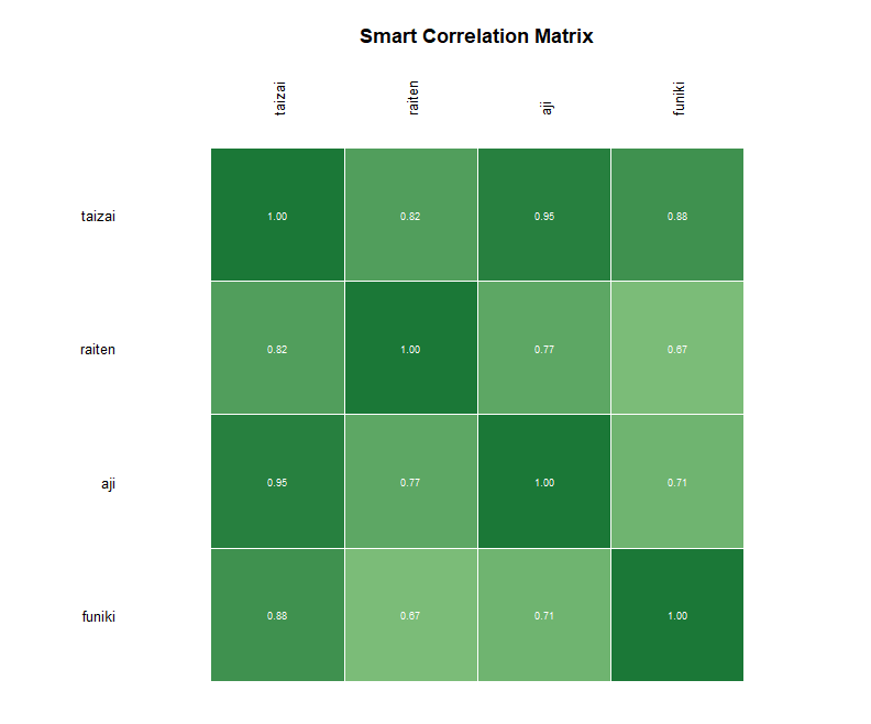
plot(mat, palette = "purple_green")

# 数値を非表示にし、配色をheatに変更してプロット
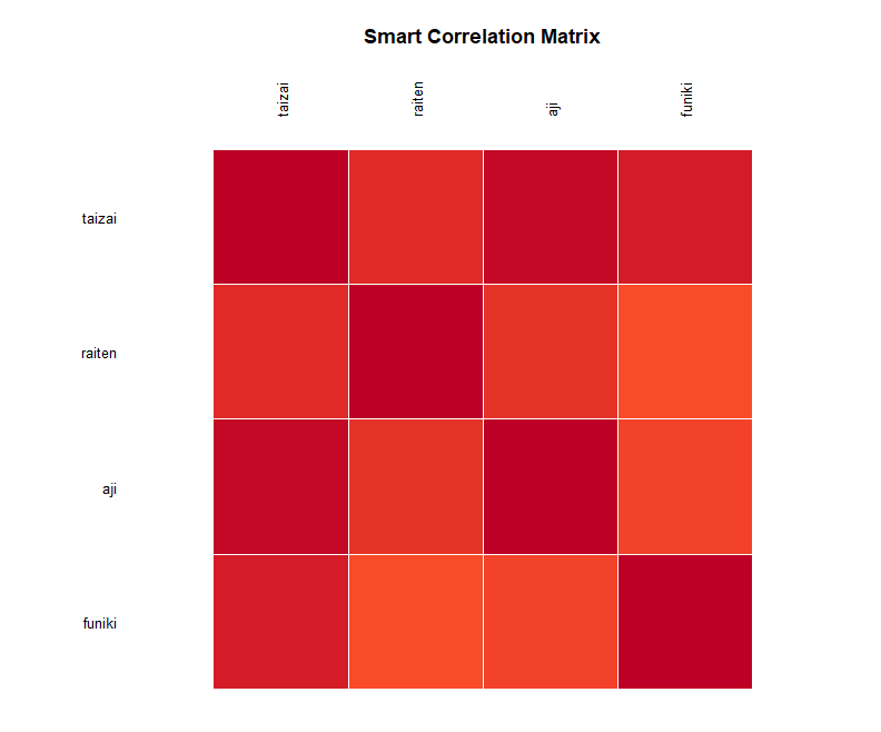
plot(mat, palette = "heat", show_values = FALSE)

# 配色をcoolに変更し、セル内の文字を1.4倍に拡大してプロット
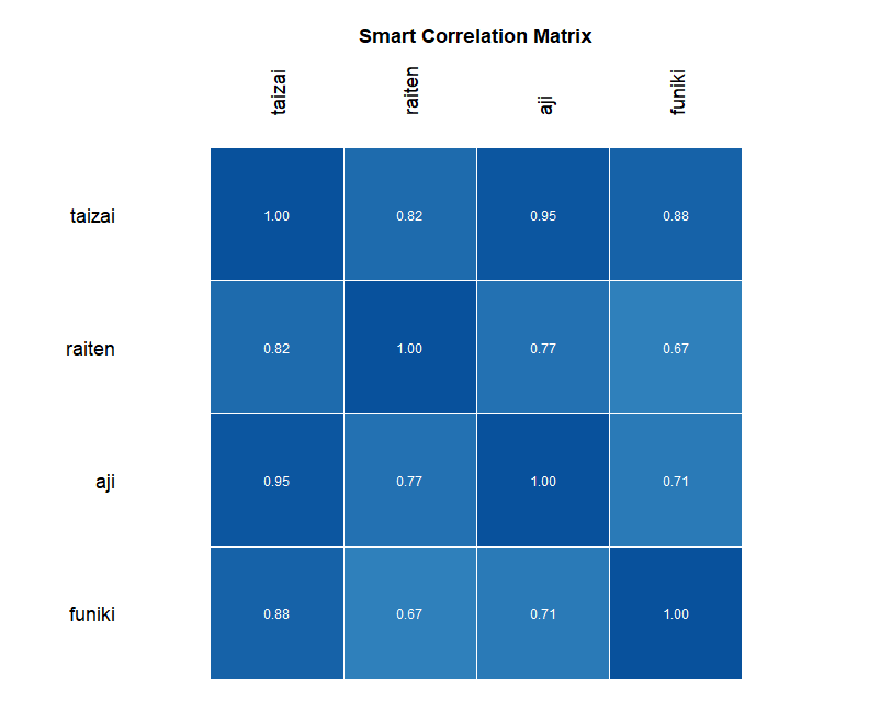
plot(mat, palette = "cool", text_size = 1.4) ・既定でヒートマップをプロット
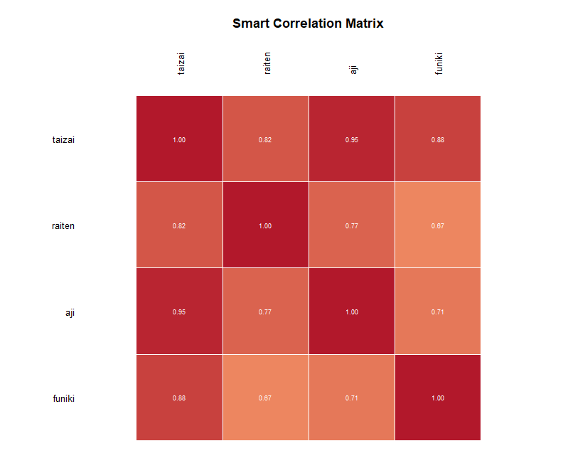
・配色を緑の配色に変更してプロット
・数値を非表示にし、配色をheatに変更してプロット
・配色をcoolに変更し、セル内の文字を1.4倍に拡大してプロット
リスト形式の結果をヒートマップでプロット:plot_cor_heatmapコマンド
| オプション | 意味 | 初期値 |
|---|---|---|
| x | 行列、数値列のみのデータフレーム、またはcorrelations要素を含む名前付きリストを指定 | なし |
| palette | “blue_red”などの文字列、または低・中・高に対応する3色のベクトルを指定 | “blue_red” |
| digits | セルに表示する小数点以下の桁数を整数で指定 | 2 |
| title | 作図のタイトル文字列またはNULLを指定 | NULL |
| show_values | 各セルに数値を表示するか否かを論理値で指定 | TRUE |
| text_size | セル内文字サイズの倍率を数値で指定 | 1 |
| … | 指定しても無視される引数 | なし |

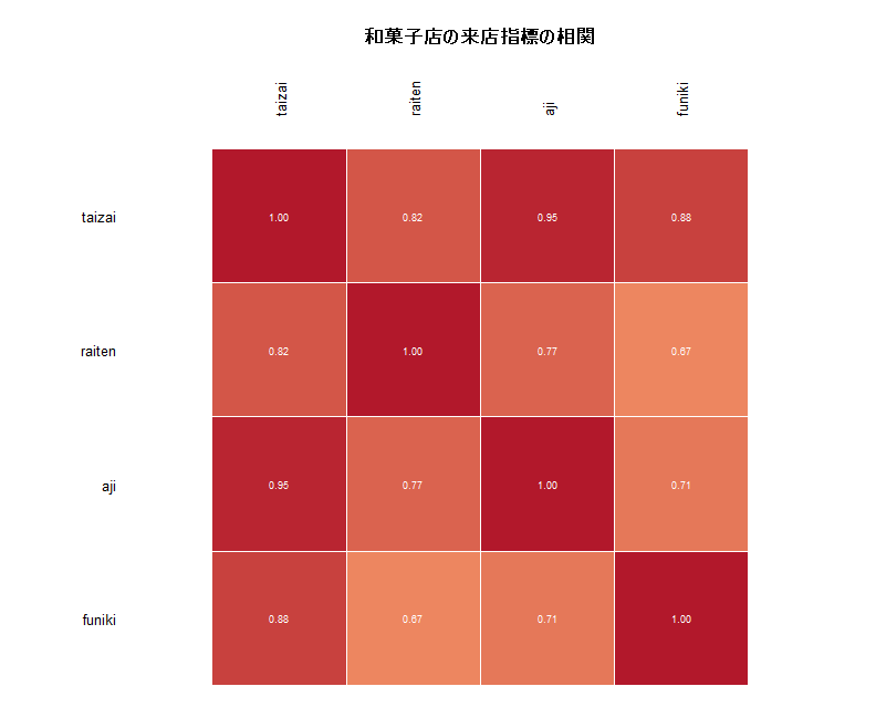
smart_cor_dfコマンドの結果や相関行列そのものを受け取ってヒートマップをプロットします。paletteに3色の文字列ベクトルを渡すと、低・中・高に対応する任意の配色を指定できます。
# 相関係数と手法をリストとして取得
kekka <- smart_cor_df(
  wagashi[, c("taizai", "raiten", "aji", "funiki")],
  assume_latent_normal = FALSE)

# リスト形式の結果からヒートマップをプロット
plot_cor_heatmap(kekka)

# 濃紺・白・濃赤の3色を指定してプロット
plot_cor_heatmap(kekka, palette = c("darkblue", "white", "darkred"))

# 相関係数のデータフレームを直接渡し、タイトルを付けてプロット
plot_cor_heatmap(kekka$correlations,
                 title = "和菓子店の来店指標の相関")
・濃紺・白・濃赤の3色を指定してプロット
ggplot2でヒートマップをプロット:ggcor_heatmapコマンド
| オプション | 意味 | 初期値 |
|---|---|---|
| x | smartcormatオブジェクト、またはcorrelations要素を含む名前付きリストを指定 | なし |
| palette | “blue_red”、”purple_green”、または低・中・高に対応する3色のベクトルを指定 | “blue_red” |
| digits | セルに表示する小数点以下の桁数を整数で指定 | 2 |
| title | 作図のタイトル文字列またはNULLを指定 | NULL |
| show_values | 各セルに数値を表示するか否かを論理値で指定 | TRUE |
| text_size | セル内文字の基準サイズを数値で指定 | 3.5 |
| lower_only | 下三角のみを表示するか否かを論理値で指定 | FALSE |
| … | 指定しても無視される引数 | なし |
ggplot2のオブジェクトなので、簡単にテーマや注釈を調整が可能です。
# 4つの変数について相関行列を作成
mat <- smart_cormat(
  wagashi[, c("taizai", "raiten", "aji", "funiki")],
  assume_latent_normal = FALSE,
  verbose = FALSE)

# 既定の配色でヒートマップをプロット
ggcor_heatmap(mat)

# 下三角部分のみを表示してプロット
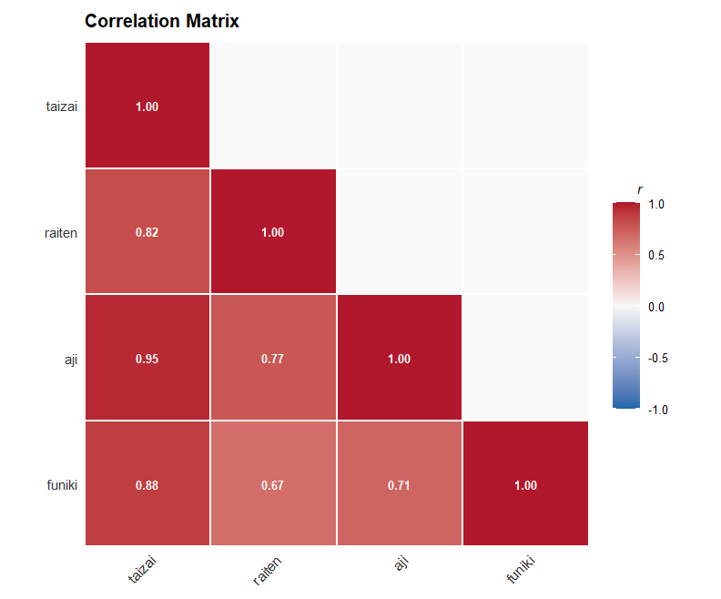
ggcor_heatmap(mat, lower_only = TRUE)

# 3色を指定し、文字サイズと小数点以下の桁数を変更してプロット
ggcor_heatmap(mat, palette = c("navy", "gray95", "firebrick"),
              text_size = 5, digits = 3)

# タイトルを指定し、ggplot2でキャプションを追加してプロット
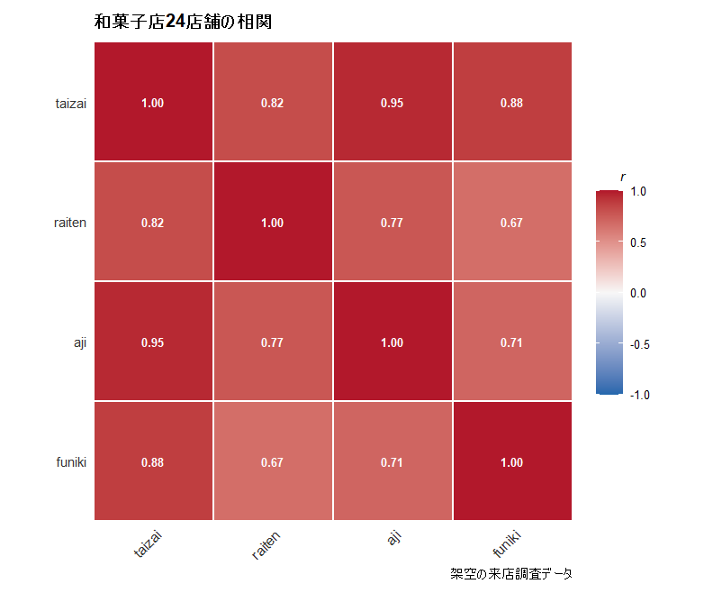
ggcor_heatmap(mat, title = "和菓子店24店舗の相関") +
  ggplot2::labs(caption = "架空の来店調査データ")
・下三角部分のみを表示してプロット

・ggplot2でタイトル、キャプションを追加してプロット
選択された手法をヒートマップでプロット:ggcor_method_heatmapコマンド
| オプション | 意味 | 初期値 |
|---|---|---|
| x | methods要素を含むsmartcormatオブジェクトまたは名前付きリストを指定 | なし |
| title | 作図のタイトル文字列またはNULLを指定 | NULL |
| show_values | 各セルに手法名を表示するか否かを論理値で指定 | TRUE |
| text_size | セル内文字の基準サイズを数値で指定 | 3.5 |
| digits | セルに表示する小数点以下の桁数を整数で指定 | 2 |
| … | 指定しても無視される引数 | なし |
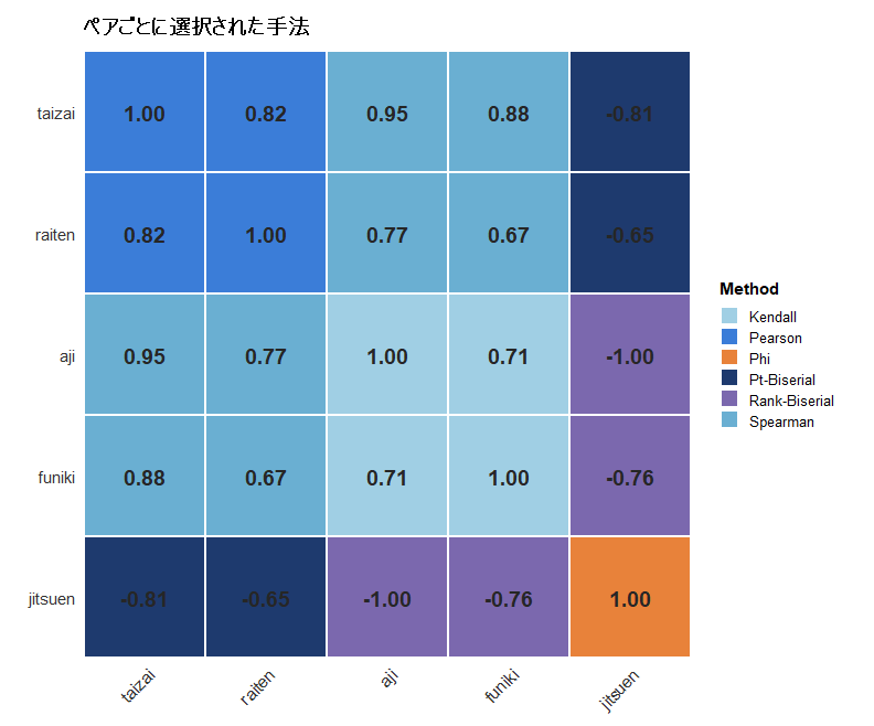
変数ペアごとに選択された手法を色分けしたヒートマップでプロットします。手法の分布を確認するのに便利です。
# 5つの変数について相関行列を作成
mat5 <- smart_cormat(
  wagashi[, c("taizai", "raiten", "aji", "funiki", "jitsuen")],
  assume_latent_normal = FALSE,
  verbose = FALSE
)
# 選択された手法をヒートマップでプロット
ggcor_method_heatmap(mat5)

# タイトルを指定し、文字サイズを大きくしてプロット
ggcor_method_heatmap(mat5, title = "ペアごとに選択された手法",
                     text_size = 5)

# 手法名を非表示にして配色のみでプロット
ggcor_method_heatmap(mat5, show_values = FALSE)
・タイトルを指定し、文字サイズを大きくしてプロット
実行例
パッケージの機能を組み合わせた、使い方の例です。結果表示とプロットは省略します。
型の確認から相関行列の作図までを一連でおこなう
変数の型を確認し、利用できる手法を把握したうえで相関行列を作成し、結果をtidyデータとヒートマップをプロットします。
# 解析対象の列を絞り込む
taisho <- wagashi[, c("taizai", "raiten", "aji", "funiki", "jitsuen", "chihou")]

# 各列の統計的タイプをまとめて確認する
kata <- vapply(taisho, detect_type, character(1))
kata

# 味の満足度と地方の組み合わせで利用できる手法を確認する
available_methods(kata[["aji"]], kata[["chihou"]])

# 潜在正規性を仮定せず、乱数シードを固定して相関行列を作成する
mat_all <- smart_cormat(
  taisho,
  assume_latent_normal = FALSE,
  seed = 20260811,
  verbose = FALSE)

# 相関行列と使用された手法を表示する
mat_all

# ペアごとの整然データへ変換する
tidy_all <- tidy(mat_all)

# 相関の絶対値が0.3以上のペアだけを抽出する
tsuyoi <- tidy_all[!is.na(tidy_all$estimate) & abs(tidy_all$estimate) >= 0.3, ]
tsuyoi[, c("var_x", "var_y", "x_type", "y_type", "method", "estimate", "p.value")]

# 相関の強弱をヒートマップで確認する
ggcor_heatmap(mat_all, lower_only = TRUE,
              title = "和菓子店24店舗の相関")

# ペアごとに選択された手法をヒートマップでプロット
ggcor_method_heatmap(mat_all, title = "選択された相関手法")
順序尺度のペアで手法の違いを比較する
順序尺度どうしの相関で仮定の妥当性を検定で確認し、手法ごとの推定値の差を並べて比較します。
# 二変量正規性を検定する
kentei <- test_bivariate_normality(wagashi$aji, wagashi$funiki)
kentei

# 潜在正規性を仮定した場合の相関を算出する
smart_cor(wagashi$aji, wagashi$funiki,
          assume_latent_normal = TRUE, verbose = FALSE)

# 潜在正規性を仮定しない場合の相関を算出する
smart_cor(wagashi$aji, wagashi$funiki,
          assume_latent_normal = FALSE, verbose = FALSE)

# 適用できる手法をすべて算出して比較する
hikaku <- compare_methods(
  wagashi$aji, wagashi$funiki,
  assume_latent_normal = FALSE,
  bootstrap = TRUE, n_boot = 1000, seed = 20260811,
  verbose = FALSE)
hikaku

# 手法ごとの推定値と信頼区間を整然データで並べる
tidy(hikaku)[, c("method", "estimate", "ci_lower", "ci_upper", "recommended")]
この記事が誰かの役に立ちますように。